.png.webp)
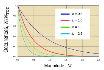
In seismology, the Gutenberg–Richter law[1] (GR law) expresses the relationship between the magnitude and total number of earthquakes in any given region and time period of at least that magnitude.
or
where
- is the number of events having a magnitude ,
- and are constants, i.e. they are the same for all values of and .
Since magnitude is logarithmic, this is an instance of the Pareto distribution.
The Gutenberg–Richter law is also widely used for acoustic emission analysis due to a close resemblance of acoustic emission phenomenon to seismogenesis.
Background
The relationship between earthquake magnitude and frequency was first proposed by Charles Francis Richter and Beno Gutenberg in a 1944 paper studying earthquakes in California,[2][3] and generalised in a worldwide study in 1949.[4] This relationship between event magnitude and frequency of occurrence is remarkably common, although the values of a and b may vary significantly from region to region or over time.

The parameter b (commonly referred to as the "b-value") is commonly close to 1.0 in seismically active regions. This means that for a given frequency of magnitude 4.0 or larger events there will be 10 times as many magnitude 3.0 or larger quakes and 100 times as many magnitude 2.0 or larger quakes. There is some variation of b-values in the approximate range of 0.5 to 2 depending on the source environment of the region.[5] A notable example of this is during earthquake swarms when b can become as high as 2.5, thus indicating a very high proportion of small earthquakes to large ones.
There is debate concerning the interpretation of some observed spatial and temporal variations of b-values. The most frequently cited factors to explain these variations are: the stress applied to the material,[6] the depth,[7] the focal mechanism,[8] the strength heterogeneity of the material,[9] and the proximity of macro-failure. The b-value decrease observed prior to the failure of samples deformed in the laboratory[10] has led to the suggestion that this is a precursor to major macro-failure.[11] Statistical physics provides a theoretical framework for explaining both the steadiness of the Gutenberg–Richter law for large catalogs and its evolution when the macro-failure is approached, but application to earthquake forecasting is currently out of reach.[12] Alternatively, a b-value significantly different from 1.0 may suggest a problem with the data set; e.g. it is incomplete or contains errors in calculating magnitude.

.svg.png.webp)
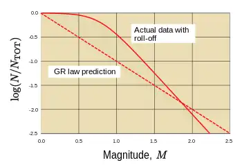
There is an apparent b-value decrease for smaller magnitude event ranges in all empirical catalogues of earthquakes. This effect is described as "roll-off" of the b-value, a description due to the plot of the logarithmic version of the GR law becoming flatter at the low magnitude end of the plot. This may in large part be caused by incompleteness of any data set due to the inability to detect and characterize small events. That is, many low-magnitude earthquakes are not catalogued because fewer stations detect and record them due to decreasing instrumental signal to noise levels. Some modern models of earthquake dynamics, however, predict a physical roll-off in the earthquake size distribution.[13]
The a-value represents the total seismicity rate of the region. This is more easily seen when the GR law is expressed in terms of the total number of events:
where
the total number of events (above M=0). Since is the total number of events, must be the probability of those events.
Modern attempts to understand the law involve theories of self-organized criticality or self similarity.
Generalization
New models show a generalization of the original Gutenberg–Richter model. Among these is the one released by Oscar Sotolongo-Costa and A. Posadas in 2004,[14] of which R. Silva et al. presented the following modified form in 2006,[15]
where N is the total number of events, a is a proportionality constant and q represents the non-extensivity parameter introduced by Constantino Tsallis to characterize systems not explained by the Boltzmann–Gibbs statistical form for equilibrium physical systems.
It is possible to see in an article published by N. V. Sarlis, E. S. Skordas, and P. A. Varotsos,[16] that above some magnitude threshold this equation reduces to original Gutenberg–Richter form with
In addition, another generalization was obtained from the solution of the generalized logistic equation.[17] In this model, values of parameter b were found for events recorded in Central Atlantic, Canary Islands, Magellan Mountains and the Sea of Japan. The generalized logistic equation is applied to acoustic emission in concrete by N. Burud and J. M. Chandra Kishen,.[18] Burud showed the b-value obtained from generalized logistic equation monotonically increases with damage and referred it as a damage compliant b-value.
A new generalization was published using Bayesian statistical techniques,[19] from which an alternative form for parameter b of Gutenberg–Richter is presented. The model was applied to intense earthquakes occurred in Chile, from the year 2010 to the year 2016.
References
- ↑ Gutenberg and Richter (1949), p. 17.
- ↑ Jamshid Ghaboussi, Michael F Insana, Understanding Systems: A Grand Challenge For 21st Century Engineering, p. 255, World Scientific, 2017 ISBN 9813225971.
- ↑ B. Gutenberg, C. F. Richter, "Frequency of Earthquakes in California", p. 186, Bulletin of the Seismological Society of America, vol. 34, iss. 4, pp. 185–188, 1944
- ↑ Gutenberg & Richter (1949), p. 17
- ↑ Bhattacharya et al, p. 120
- ↑ Scholz, C. H. (1968), the frequency-magnitude relation of microfracturing in rock and its relation to earthquakes, BSSA, 58(1), 399–415.
- ↑ Mori, J., et R. E. Abercombie (1997), Depth dependence of earthquake frequency-magnitude distributions in California: Implication for rupture initiation, Journal of Geophysical Research, 102(B7), 15081–15090.
- ↑ Schorlemmer, D., S. Wiemer, et M. Wyss (2005), Variations in earthquake-size distribution across different stress regimes, Nature, 437, 539–542, doi: 10.1038/nature04094.
- ↑ Mogi, K. (1962), Magnitude frequency relations for elastic shocks accompanying fractures of various materials and some related problems in earthquakes, Bull. Earthquake Res. Inst. Univ. Tokyo, 40, 831–853.
- ↑ Lockner, D. A., et J. D. Byerlee (1991), Precursory AE patterns leading to rock fracture, in Vth Conf. AE/MS Geol. Str. and Mat., édité par Hardy, pp. 45–58, Trans Tech Publication, Germany, The pennsylvania State University.
- ↑ Smith, W. D. (1981), The b-value as an earthquake precursor, Nature, 289, 136–139; doi:10.1038/289136a0.
- ↑ Amitrano, D. (2012), Variability in the power-law distributions of rupture events, how and why does b-value change, Eur. Phys. J.-Spec. Top., 205(1), 199–215, doi:10.1140/epjst/e2012-01571-9.
- ↑ Bhattacharya et al, pp. 119–121
Pelletier, pp. 34–36. - ↑ Sotolongo-Costa O., Posadas A., "Fragment-Asperity Interaction Model for Earthquakes", Phys. Rev. Lett. 92 (2004) 048501.
- ↑ Silva R., Franca G.S., Vilar C.S., Alcaniz J.S., "Nonextensive models for earthquakes", Phys. Rev. E 73 (2006) 026102.
- ↑ N. V. Sarlis, E. S. Skordas, and P. A. Varotsos, "Nonextensivity and natural time: The case of seismicity", Physical Review E 82 (2010), 021110.
- ↑ Lev A. Maslov and Vladimir M. Anokhin, "Derivation of the Gutenberg-Richter empirical formula from the solution of the generalized logistic equation", Natural Science, 04, 08, (648), (2012).
- ↑ Burud, Nitin B; Kishen, J M Chandra. "Application of generalized logistic equation for b-value analysis in fracture of plain concrete beams under flexure", Engineering Fracture Mechanics Vol 210, 2019, pp. 228–246. doi:10.1016/j.engfracmech.2018.09.011
- ↑ Sanchez E; Vega-Jorquera P. "New Bayesian frequency–magnitude distribution model for earthquakes applied in Chile", Physica A: Stat. Mech. and its Appl. Vol 508, 2018, pp. 305–312. doi:10.1016/j.physa.2018.05.119
Bibliography
- Pathikrit Bhattacharya, Bikas K Chakrabarti, Kamal, and Debashis Samanta, "Fractal models of earthquake dynamics", Heinz Georg Schuster (ed), Reviews of Nonlinear Dynamics and Complexity, pp. 107–150 V.2, Wiley-VCH, 2009 ISBN 3-527-40850-9.
- B. Gutenberg and C. F. Richter, Seismicity of the Earth and Associated Phenomena, Princeton University Press, 1949 OCLC 1323229850.
- Jon D. Pelletier, "Spring-block models of seismicity: review and analysis of a structurally heterogeneous model coupled to the viscous asthenosphere" Geocomplexity and the Physics of Earthquakes, American Geophysical Union, 2000 ISBN 0-87590-978-7.