In information theory and machine learning, information gain is a synonym for Kullback–Leibler divergence; the amount of information gained about a random variable or signal from observing another random variable. However, in the context of decision trees, the term is sometimes used synonymously with mutual information, which is the conditional expected value of the Kullback–Leibler divergence of the univariate probability distribution of one variable from the conditional distribution of this variable given the other one.

The information gain of a random variable X obtained from an observation of a random variable A taking value ${\displaystyle A=a}$ is defined

$${\displaystyle IG_{X,A}{(X,a)}=D_{\text{KL}}{\left(P_{X}{(x|a)}\|P_{X}{(x|I)}\right)},}$$

the Kullback–Leibler divergence of the prior distribution ${\displaystyle P_{X}{(x|I)}}$ for x from the posterior distribution ${\displaystyle P_{X|A}{(x|a)}}$ for x given a.

The expected value of the information gain is the mutual information ${\displaystyle I(X;A)}$ of X and A – i.e. the reduction in the entropy of X achieved by learning the state of the random variable A.

In machine learning, this concept can be used to define a preferred sequence of attributes to investigate to most rapidly narrow down the state of X. Such a sequence (which depends on the outcome of the investigation of previous attributes at each stage) is called a decision tree and applied in the area of machine learning known as decision tree learning. Usually an attribute with high mutual information should be preferred to other attributes.

General definition

In general terms, the expected information gain is the reduction in information entropy Η from a prior state to a state that takes some information as given:

${\displaystyle IG(T,a)=\mathrm {H} {(T)}-\mathrm {H} {(T|a)},}$

where ${\displaystyle \mathrm {H} {(T|a)}}$ is the conditional entropy of ${\displaystyle T}$ given the value of attribute ${\displaystyle a}$.

This is intuitively plausible when interpreting entropy Η as a measure of uncertainty of a random variable ${\displaystyle T}$: by learning (or assuming) ${\displaystyle a}$ about ${\displaystyle T}$, our uncertainty about ${\displaystyle T}$ is reduced (i.e. ${\displaystyle IG(T,a)}$ is positive), unless of course ${\displaystyle T}$ is independent of ${\displaystyle a}$, in which case ${\displaystyle \mathrm {H} (T,a)=\mathrm {H} (T)}$, meaning ${\displaystyle IG(T,a)=0}$.

Formal definition

Let T denote a set of training examples, each of the form ${\displaystyle ({\textbf {x}},y)=(x_{1},x_{2},x_{3},...,x_{k},y)}$ where ${\displaystyle x_{a}\in \mathrm {vals} (a)}$ is the value of the ${\displaystyle a^{\text{th}}}$ attribute or feature of example ${\displaystyle {\textbf {x}}}$ and y is the corresponding class label. The information gain for an attribute a is defined in terms of Shannon entropy ${\displaystyle \mathrm {H} (-)}$ as follows. For a value v taken by attribute a, let

$${\displaystyle S_{a}{(v)}=\{{\textbf {x}}\in T|x_{a}=v\}}$$

be defined as the set of training inputs of T for which attribute a is equal to v. Then the information gain of T for attribute a is the difference between the a priori Shannon entropy ${\displaystyle \mathrm {H} (T)}$ of the training set and the conditional entropy ${\displaystyle \mathrm {H} {(T|a)}}$.

$${\displaystyle \mathrm {H} (T|a)=\sum _{v\in \mathrm {vals} (a)}{{\frac {|S_{a}{(v)}|}{|T|}}\cdot \mathrm {H} \left(S_{a}{\left(v\right)}\right)}.}$$

${\displaystyle IG(T,a)=\mathrm {H} (T)-\mathrm {H} (T|a)}$

The mutual information is equal to the total entropy for an attribute if for each of the attribute values a unique classification can be made for the result attribute. In this case, the relative entropies subtracted from the total entropy are 0. In particular, the values ${\displaystyle v\in vals(a)}$ defines a partition of the training set data T into mutually exclusive and all-inclusive subsets, inducing a categorical probability distribution ${\textstyle P_{a}{(v)}}$ on the values ${\textstyle v\in vals(a)}$ of attribute a. The distribution is given ${\textstyle P_{a}{(v)}:={\frac {|S_{a}{(v)}|}{|T|}}}$. In this representation, the information gain of T given a can be defined as the difference between the unconditional Shannon entropy of T and the expected entropy of T conditioned on a, where the expectation value is taken with respect to the induced distribution on the values of a.

$${\displaystyle {\begin{alignedat}{2}IG(T,a)&=\mathrm {H} (T)-\sum _{v\in \mathrm {vals} (a)}{P_{a}{(v)}\mathrm {H} \left(S_{a}{(v)}\right)}\\&=\mathrm {H} (T)-\mathbb {E} _{P_{a}}{\left[\mathrm {H} {(S_{a}{(v)})}\right]}\\&=\mathrm {H} (T)-\mathrm {H} {(T|a)}.\end{alignedat}}}$$

Another Take on Information Gain, with Example

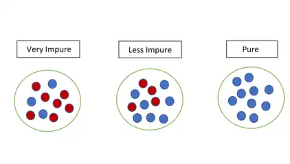
For a better understanding of information gain, let us break it down. As we know, information gain is the reduction in information entropy, what is entropy? Basically, entropy is the measure of impurity or uncertainty in a group of observations. In engineering applications, information is analogous to signal, and entropy is analogous to noise. It determines how a decision tree chooses to split data.^[1] The leftmost figure below is very impure and has high entropy corresponding to higher disorder and lower information value. As we go to the right, the entropy decreases, and the information value increases.

Entropy diagram^[2]

A simple decision tree

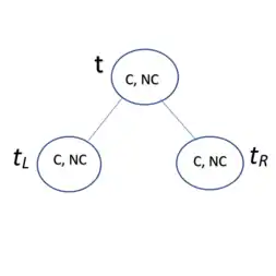
Now, it is clear that information gain is the measure of how much information a feature provides about a class. Let's visualize information gain in a decision tree as shown in the right:

The node t is the parent node, and the sub-nodes t_L and t_R are child nodes. In this case, the parent node t has a collection of cancer and non-cancer samples denoted as C and NC respectively. We can use information gain to determine how good the splitting of nodes is in a decision tree. In terms of entropy, information gain is defined as:

Gain = (Entropy of the parent node) – (average entropy of the child nodes)[2]

(i)

To understand this idea, let's start by an example in which we create a simple dataset and want to see if gene mutations could be related to patients with cancer. Given four different gene mutations, as well as seven samples, the training set for a decision can be created as follows:

In this dataset, a 1 means the sample has the mutation (True), while a 0 means the sample does not (False). A sample with C denotes that it has been confirmed to be cancerous, while NC means it is non-cancerous. Using this data, a decision tree can be created with information gain used to determine the candidate splits for each node.

For the next step, the entropy at parent node t of the above simple decision tree is computed as:

H(t) = −[p_C,t log₂(p_C,t) + p_NC,t log₂(p_NC,t)]^[3]

where,

probability of selecting a class ‘C’ sample at node t, p_C,t = n(t, C) / n(t),

probability of selecting a class ‘NC’ sample at node t, p_NC,t = n(t, NC) / n(t),

n(t), n(t, C), and n(t, NC) are the number of total samples, ‘C’ samples and ‘NC’ samples at node t respectively.

Using this with the example training set, the process for finding information gain beginning with ${\displaystyle \mathrm {H} {(t)}}$ for Mutation 1 is as follows:

p_{C, t} = 4/7

p_{NC, t} = 3/7

${\displaystyle \mathrm {H} {(t)}}$ = −(4/7 × log₂(4/7) + 3/7 × log₂(3/7)) = 0.985

Note: ${\displaystyle \mathrm {H} {(t)}}$ will be the same for all mutations at the root.

The relatively high value of entropy ${\displaystyle \mathrm {H} {(t)}=0.985}$ (1 is the optimal value) suggests that the root node is highly impure and the constituents of the input at the root node would look like the leftmost figure in the above Entropy Diagram. However, such a set of data is good for learning the attributes of the mutations used to split the node. At a certain node, when the homogeneity of the constituents of the input occurs (as shown in the rightmost figure in the above Entropy Diagram), the dataset would no longer be good for learning.

Moving on, the entropy at left and right child nodes of the above decision tree is computed using the formulae:

H(t_L) = −[p_C,L log₂(p_C,L) + p_NC,L log₂(p_NC,L)]^[1]

H(t_R) = −[p_C,R log₂(p_C,R) + p_NC,R log₂(p_NC,R)]^[1]

where,

probability of selecting a class ‘C’ sample at the left child node, p_C,L = n(t_L, C) / n(t_L),

probability of selecting a class ‘NC’ sample at the left child node, p_NC,L = n(t_L, NC) / n(t_L),

probability of selecting a class ‘C’ sample at the right child node, p_C,R = n(t_R, C) / n(t_R),

probability of selecting a class ‘NC’ sample at the right child node, p_NC,R = n(t_R, NC) / n(t_R),

n(t_L), n(t_L, C), and n(t_L, NC) are the total number of samples, ‘C’ samples and ‘NC’ samples at the left child node respectively,

n(t_R), n(t_R, C), and n(t_R, NC) are the total number of samples, ‘C’ samples and ‘NC’ samples at the right child node respectively.

Using these formulae, the H(t_L) and H(t_R) for Mutation 1 is shown below:

H(t_L) = −(3/4 × log₂(3/4) + 1/4 × log₂(1/4)) = 0.811

H(t_R) = −(1/3 × log₂(1/3) + 2/3 × log₂(2/3)) = 0.918

Following this, average entropy of the child nodes due to the split at node t of the above decision tree is computed as:

H(s,t) = P_LH(t_L) + P_RH(t_R)

where,

probability of samples at the left child, P_L = n(t_L) / n(t),

probability of samples at the right child, P_R = n(t_R) / n(t),

Finally, H(s,t) along with P_L and P_R for Mutation 1 is as follows:

P_L = 4/7

P_R = 3/7

H(s, t) = (4/7 × 0.811) + (3/7 × 0.918) = 0.857

Thus, by definition from equation (i):

(Information gain) = H(t) - H(s,t)

After all the steps, gain(s), where s is a candidate split for the example is:

gain(s) = 0.985 – 0.857 = 0.128

The newly created tree with the root node split based on Mutation 3. Mutation 3 had the highest information gain, so it was selected as the split.

Using this same set of formulae with the other three mutations leads to a table of the candidate splits, ranked by their information gain:

The mutation that provides the most useful information would be Mutation 3, so that will be used to split the root node of the decision tree. The root can be split and all the samples can be passed though and appended to the child nodes. A tree describing the split is shown on the left.

The samples that are on the left node of the tree would be classified as cancerous by the tree, while those on the right would be non-cancerous. This tree is relatively accurate at classifying the samples that were used to build it (which is a case of overfitting), but it would still classify sample C2 incorrectly. To remedy this, the tree can be split again at the child nodes to possibly achieve something even more accurate.

To split the right node, information gain must again be calculated for all the possible candidate splits that were not used for previous nodes. So, the only options this time are Mutations 1, 2, and 4.

Note: ${\displaystyle \mathrm {H} {(t)}}$ is different this time around since there are only four samples at the right child.

P_{C, t} = 1/4

P_{NC, t} = 3/4

${\displaystyle \mathrm {H} {(t)}}$ = -(1/4 × log₂(1/4) + 3/4 × log₂(3/4)) = 0.811

The updated tree with the right child node split based on Mutation 4.

From this new ${\displaystyle \mathrm {H} {(t)}}$, the candidate splits can be calculated using the same formulae as the root node:

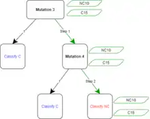
Thus, the right child will be split with Mutation 4. All the samples that have the mutation will be passed to the left child and the ones that lack it will be passed to the right child.

To split the left node, the process would be the same, except there would only be 3 samples to check. Sometimes a node may not need to be split at all if it is a pure set, where all samples at the node are just cancerous or non-cancerous. Splitting the node may lead to the tree being more inaccurate and in this case it will not be split.

The tree would now achieve 100% accuracy if the samples that were used to build it are tested. This isn't a good idea, however, since the tree would overfit the data. The best course of action is to try testing the tree on other samples, of which are not part of the original set. Two outside samples are below:

Testing the decision tree with two new samples.

By following the tree, NC10 was classified correctly, but C15 was classified as NC. For other samples, this tree would not be 100% accurate anymore. It could be possible to improve this though, with options such as increasing the depth of the tree or increasing the size of the training set.

Advantages

Information gain is the basic criterion to decide whether a feature should be used to split a node or not. The feature with the optimal split i.e., the highest value of information gain at a node of a decision tree is used as the feature for splitting the node.

The concept of information gain function falls under the C4.5 algorithm for generating the decision trees and selecting the optimal split for a decision tree node.^[1] Some of its advantages include:

• It can work with both continuous and discrete variables.
• Due to the factor –[p ∗ log(p)] in the entropy definition as given above, leaf nodes with a small number of instances are assigned less weight and it favors dividing rest of the data into bigger but homogeneous groups. And thus, as we dig deeper into the depth of the tree, the dataset becomes more homogeneous. This approach is usually more stable and chooses the most impactful features on the nodes.^[4]

Drawbacks and Solutions

Although information gain is usually a good measure for deciding the relevance of an attribute, it is not perfect. A notable problem occurs when information gain is applied to attributes that can take on a large number of distinct values. For example, suppose that one is building a decision tree for some data describing the customers of a business. Information gain is often used to decide which of the attributes are the most relevant, so they can be tested near the root of the tree. One of the input attributes might be the customer's membership number, if they are a member of the business's membership program. This attribute has a high mutual information, because it uniquely identifies each customer, but we do not want to include it in the decision tree. Deciding how to treat a customer based on their membership number is unlikely to generalize to customers we haven't seen before (overfitting). This issue can also occur if the samples that are being tested have multiple attributes with many distinct values. In this case, it can cause the information gain of each of these attributes to be much higher than those without as many distinct values.

To counter this problem, Ross Quinlan proposed to instead choose the attribute with highest information gain ratio from among the attributes whose information gain is average or higher.^[5] This biases the decision tree against considering attributes with a large number of distinct values, while not giving an unfair advantage to attributes with very low information value, as the information value is higher or equal to the information gain.^[6]

See also

• Information gain more broadly
• Decision tree learning
• Information content, the starting point of information theory and the basis of Shannon entropy
• Information gain ratio
• ID3 algorithm
  • C4.5 algorithm
• Surprisal analysis

References

Further reading

• Nowozin, Sebastion (2012-06-18). "Improved Information Gain Estimates for Decision Tree Induction". arXiv:1206.4620v1.
• Shouman, Mai (2011). "Using decision tree for diagnosing heart disease patients" (PDF). Proceedings of the Ninth Australasian Data Mining Conference. 121: 23–30.
• Mitchell, Tom M. (1997). Machine Learning. The Mc-Graw-Hill Companies, Inc. ISBN 978-0070428072.

References

- 1 2 3 4 Larose, Daniel T. (2014). Discovering Knowledge in Data: An Introduction to Data Mining. Hoboken, New Jersey: Wiley. pp. 174–179. ISBN 9780470908747.
- 1 2 Gopalan, Bhuvaneswari (2020-12-10). "What is Entropy and Information Gain? How are they used to construct decision trees?". Numpy Ninja. Retrieved 2021-11-28.
- ↑ Jothikumar, R. (2018). "Predicting Life time of Heart Attack Patient using Improved C4.5 Classification Algorithm". Research Journal of Pharmacy and Technology. 11 (5): 1951–1956. doi:10.5958/0974-360X.2018.00362.1.
- ↑ "machine learning - Why we use information gain over accuracy as splitting criterion in decision tree?". Data Science Stack Exchange. Retrieved 2021-12-09.
- ↑ Quinlan, J. Ross (1986). "Induction of Decision Trees". Machine Learning. 1 (1): 81–106. doi:10.1007/BF00116251.
- ↑ Milman, Oren (August 6, 2018). "What is the range of information gain ratio?". Stack Exchange. Retrieved 2018-10-09.