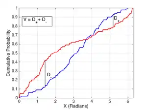
Kuiper's test is used in statistics to test that whether a given distribution, or family of distributions, is contradicted by evidence from a sample of data. It is named after Dutch mathematician Nicolaas Kuiper.[1]
Kuiper's test is closely related to the better-known Kolmogorov–Smirnov test (or K-S test as it is often called). As with the K-S test, the discrepancy statistics D+ and D− represent the absolute sizes of the most positive and most negative differences between the two cumulative distribution functions that are being compared. The trick with Kuiper's test is to use the quantity D+ + D− as the test statistic. This small change makes Kuiper's test as sensitive in the tails as at the median and also makes it invariant under cyclic transformations of the independent variable. The Anderson–Darling test is another test that provides equal sensitivity at the tails as the median, but it does not provide the cyclic invariance.
This invariance under cyclic transformations makes Kuiper's test invaluable when testing for cyclic variations by time of year or day of the week or time of day, and more generally for testing the fit of, and differences between, circular probability distributions.
Definition

The test statistic, V, for Kuiper's test is defined as follows. Let F be the continuous cumulative distribution function which is to be the null hypothesis. Denote the sample of data which are independent realisations of random variables, having F as their distribution function, by xi (i=1,...,n). Then define[2]
and finally,
Tables for the critical points of the test statistic are available,[3] and these include certain cases where the distribution being tested is not fully known, so that parameters of the family of distributions are estimated.
Example
We could test the hypothesis that computers fail more during some times of the year than others. To test this, we would collect the dates on which the test set of computers had failed and build an empirical distribution function. The null hypothesis is that the failures are uniformly distributed. Kuiper's statistic does not change if we change the beginning of the year and does not require that we bin failures into months or the like.[1][4] Another test statistic having this property is the Watson statistic,[2][4] which is related to the Cramér–von Mises test.
However, if failures occur mostly on weekends, many uniform-distribution tests such as K-S and Kuiper would miss this, since weekends are spread throughout the year. This inability to distinguish distributions with a comb-like shape from continuous uniform distributions is a key problem with all statistics based on a variant of the K-S test. Kuiper's test, applied to the event times modulo one week, is able to detect such a pattern. Using event times that have been modulated with the K-S test can result in different results depending on how the data is phased. In this example, the K-S test may detect the non-uniformity if the data is set to start the week on Saturday, but fail to detect the non-uniformity if the week starts on Wednesday.
See also
References
- 1 2 Kuiper, N. H. (1960). "Tests concerning random points on a circle". Proceedings of the Koninklijke Nederlandse Akademie van Wetenschappen, Series A. 63: 38–47.
- 1 2 Pearson, E.S., Hartley, H.O. (1972) Biometrika Tables for Statisticians, Volume 2, CUP. ISBN 0-521-06937-8 (page 118)
- ↑ Pearson, E.S., Hartley, H.O. (1972) Biometrika Tables for Statisticians, Volume 2, CUP. ISBN 0-521-06937-8 (Table 54)
- 1 2 Watson, G.S. (1961) "Goodness-Of-Fit Tests on a Circle", Biometrika, 48 (1/2), 109–114 JSTOR 2333135