In computer graphics, marching squares is an algorithm that generates contours for a two-dimensional scalar field (rectangular array of individual numerical values). A similar method can be used to contour 2D triangle meshes.
The contours can be of two kinds:
- Isolines – lines following a single data level, or isovalue.
- Isobands – filled areas between isolines.
Typical applications include the contour lines on topographic maps or the generation of isobars for weather maps.
Marching squares takes a similar approach to the 3D marching cubes algorithm:
- Process each cell in the grid independently.
- Calculate a cell index using comparisons of the contour level(s) with the data values at the cell corners.
- Use a pre-built lookup table, keyed on the cell index, to describe the output geometry for the cell.
- Apply linear interpolation along the boundaries of the cell to calculate the exact contour position.
Basic algorithm
Here are the steps of the algorithm:
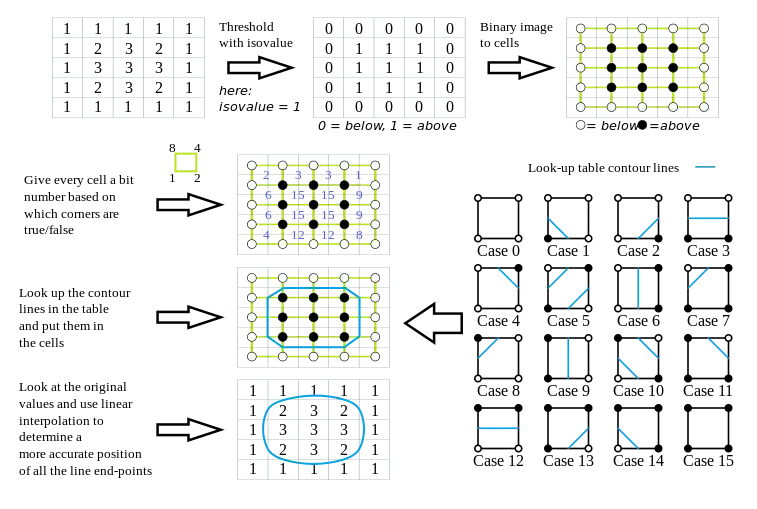
Apply a threshold to the 2D field to make a binary image containing:
- 1 where the data value is above the isovalue
- 0 where the data value is below the isovalue
Note: Data equal to the isovalue has to be treated as above or below in a consistent way.
Every 2x2 block of pixels in the binary image forms a contouring cell, so the whole image is represented by a grid of such cells (shown in green in the picture below). Note that this contouring grid is one cell smaller in each direction than the original 2D field.
For each cell in the contouring grid:
- Compose the 4 bits at the corners of the cell to build a binary index: walk around the cell in a clockwise direction appending the bit to the index, using bitwise OR and left-shift, from most significant bit at the top left, to least significant bit at the bottom left. The resulting 4-bit index can have 16 possible values in the range 0–15.
- Use the cell index to access a pre-built lookup table with 16 entries listing the edges needed to represent the cell (shown in the lower right part of the picture below).
- Apply linear interpolation between the original field data values to find the exact position of the contour line along the edges of the cell.
Disambiguation of saddle points
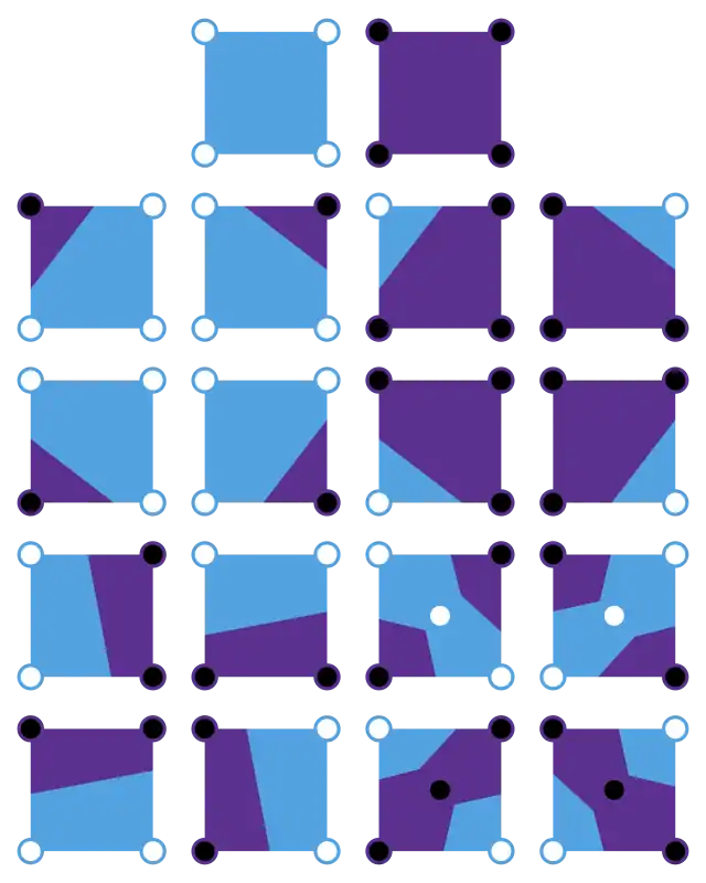
The contour is ambiguous at saddle points. It is possible to resolve the ambiguity by using the average data value for the center of the cell to choose between different connections of the interpolated points (four images in bottom-right corner):
Isobands
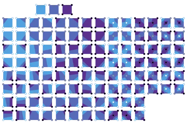
A similar algorithm can be created for filled contour bands within upper and lower threshold values:
Contouring triangle meshes
The same basic algorithm can be applied to triangular meshes, which consist of connected triangles with data assigned to the vertices. For example, a scattered set of data points could be connected with a Delaunay triangulation to allow the data field to be contoured.
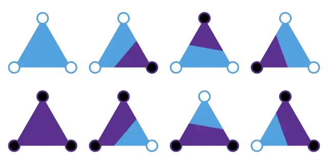
A triangular cell is always planar, because it is a 2-simplex (i.e. specified by n+1 vertices in an n-dimensional space). There is always a unique linear interpolant across a triangle, and no possibility of an ambiguous saddle.
Isolines
The analysis for isolines over triangles is especially simple: there are 3 binary digits, so there are 8 possibilities:
Isobands
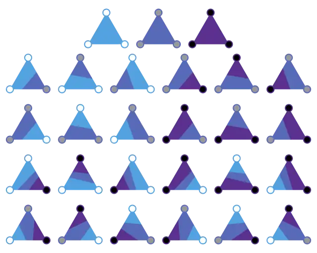
The analysis for isobands over triangles requires 3 ternary trits, so there are 27 possibilities:
Dimensions and spaces
The data space for the Marching Squares algorithm is 2D, because the vertices assigned a data value are connected to their neighbors in a 2D topological grid, but the spatial coordinates assigned to the vertices can be in 2D, 3D or higher dimensions.
For example, a triangular mesh may represent a 2D data surface embedded in 3D space, where spatial positions of the vertices and interpolated points along a contour will all have 3 coordinates. Note that the case of squares is ambiguous again, because a quadrilateral embedded in 3-dimensional space is not necessarily planar, so there is a choice of geometrical interpolation scheme to draw the banded surfaces in 3D.
Performance considerations
The algorithm is embarrassingly parallel, because all cells are processed independently. It is easy to write a parallel algorithm assuming:
- Shared read-only input scalar field.
- Shared append-only geometry output stream.
A naive implementation of Marching Squares that processes every cell independently will perform every linear interpolation twice (isoline) or four times (isoband). Similarly, the output will contain 2 copies of the 2D vertices for disjoint lines (isoline) or 4 copies for polygons (isobands). [Under the assumptions that: the grid is large, so that most cells are internal; and a full contiguous set of isobands is being created.]
It is possible to reduce the computational overhead by caching the results of interpolation. For example, a single-threaded serial version would only need to cache interpolated results for one row of the input grid.
It is also possible to reduce the size of the output by using indexed geometric primitives, i.e. create an array of 2D vertices and specify lines or polygons with short integer offsets into the array.
References
- Maple, C. (2003). "Geometric design and space planning using the marching squares and marching cube algorithms". 2003 International Conference on Geometric Modeling and Graphics, 2003. Proceedings. pp. 90–95. doi:10.1109/GMAG.2003.1219671. ISBN 978-0-7695-1985-2. S2CID 11320513.
{{cite book}}:|journal=ignored (help) - Banks, D. C. (2004). "Counting cases in substitope algorithms". IEEE Trans. Visual. Comp. Graphics. 10 (4): 371–384. CiteSeerX 10.1.1.582.7221. doi:10.1109/TVCG.2004.6. PMID 18579966. S2CID 2450480.
- Laguardia, J. J.; Cueto, E.; Doblaré, M. (2005). "A natural neighbour Galerkin method with quadtree structure". Int. J. Numer. Methods Eng. 63 (6): 789–812. Bibcode:2005IJNME..63..789L. doi:10.1002/nme.1297. S2CID 122746298.
- Schaefer, Scott; Warren, Joe (2005). "Dual marching cubes: primal contouring of dual grids". Computer Graphics Forum. 24 (2): 195–201. doi:10.1111/j.1467-8659.2005.00843.x. S2CID 10015045.
- Mantz, Huber; Jacobs, Karin; Mecke, Klaus (2008). "Utilizing Minkowski functionals for image analysis: a marching square algorithm". J. Stat. Mech.: Theory Exp. 2008 (12): P12015. Bibcode:2008JSMTE..12..015M. doi:10.1088/1742-5468/2008/12/P12015. S2CID 122873298.
- Cipolletti, Marina P.; Delrieux, Claudio A.; Perillo, Gerardo M. E.; Piccolo, M. Cintia (2012). "Superresolution border segmentation and measurement in remote sensing images". Comp. Geosci. 40: 87–97. Bibcode:2012CG.....40...87C. doi:10.1016/j.cageo.2011.07.015.
External links
- Marching Square Matlab algorithm – An easy to understand open-source marching square algorithm.
- implementation in Java
- Marching Squares code in Java. Given a 2D data set and thresholds, returns GeneralPath[] for easy plotting.
- Meandering Triangles explanation and sample Python implementation.
- Marching Squares code in C – A single header library for marching squares that can export triangle meshes for easy rendering.