Time–frequency analysis for music signals is one of the applications of time–frequency analysis. Musical sound can be more complicated than human vocal sound, occupying a wider band of frequency. Music signals are time-varying signals; while the classic Fourier transform is not sufficient to analyze them, time–frequency analysis is an efficient tool for such use. Time–frequency analysis is extended from the classic Fourier approach. Short-time Fourier transform (STFT), Gabor transform (GT) and Wigner distribution function (WDF) are famous time–frequency methods, useful for analyzing music signals such as notes played on a piano, a flute or a guitar.
Knowledge about music signal
Music is a type of sound that has some stable frequencies in a time period. Music can be produced by several methods. For example, the sound of a piano is produced by striking strings, and the sound of a violin is produced by bowing. All musical sounds have their fundamental frequency and overtones. Fundamental frequency is the lowest frequency in harmonic series. In a periodic signal, the fundamental frequency is the inverse of the period length. Overtones are integer multiples of the fundamental frequency.
Table. 1 the fundamental frequency and overtone Frequency Order f = 440 Hz N = 1 Fundamental frequency 1st harmonic f = 880 Hz N = 2 1st overtone 2nd harmonic f = 1320 Hz N = 3 2nd overtone 3rd harmonic f = 1760 Hz N = 4 3rd overtone 4th harmonic
In musical theory, pitch represents the perceived fundamental frequency of a sound. However the actual fundamental frequency may differ from the perceived fundamental frequency because of overtones.
Short-time Fourier transform


Continuous STFT
Short-time Fourier transform is a basic type of time–frequency analysis. If there is a continuous signal x(t), we can compute the short-time Fourier transform by
where w(t) is a window function. When the w(t) is a rectangular function, the transform is called Rec-STFT. When the w(t) is a Gaussian function, the transform is called Gabor transform.
Discrete STFT
However, normally the musical signal we have is not a continuous signal. It is sampled in a sampling frequency. Therefore, we can’t use the formula to compute the Rec-short-time Fourier transform. We change the original form to
Let , , and . There are some constraints of discrete short-time Fourier transform:
- where N is an integer.
- , where is the highest frequency in the signal.
STFT example
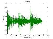
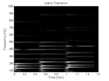
Figure 1 shows the waveform of an audio file "" with 44100 Hz sampling frequency. Figure 2 shows the time-frequency plot of the short-time Fourier transform (in particular, Gabor transform) results of the audio file. In this plot, horizontal lines with frequencies not greater than 230 Hz represent the fundamental frequencies while horizontal lines with frequencies above 230 Hz represent the harmonic components. Observe that from t = 0 to 0.5 second, a chord consists of three notes (C-E-G) is played. The chord then changed to C-E-A at t = 0.5, and then changed again to D-F-A at t = 1.
Spectrogram
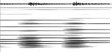
Figure 3 shows the spectrogram of the audio file shown in Figure 1. Spectrogram is the square of STFT, time-varying spectral representation. The spectrogram of a signal s(t) can be estimated by computing the squared magnitude of the STFT of the signal s(t), as shown below:
Although the spectrogram is profoundly useful, it still has one drawback. It displays frequencies on a uniform scale. However, musical scales are based on a logarithmic scale for frequencies. Therefore, we should describe the frequency in logarithmic scale related to human hearing.
Wigner distribution function
The Wigner distribution function can also be used to analyze music signals. The advantage of the Wigner distribution function is the high clarity of the output; however, it is computationally expensive and has a cross-term problem, so it's more suitable to analyze signals without more than one frequency at the same time.
Formula
The Wigner distribution function is:
where x(t) is the signal, and x*(t) is the conjugate of the signal.
See also
Sources
- Joan Serra, Emilia Gomez, Perfecto Herrera, and Xavier Serra, "Chroma Binary Similarity and Local Alignment Applied to Cover Song Identification," August, 2008
- William J. Pielemeier, Gregory H. Wakefield, and Mary H. Simoni, "Time–frequency Analysis of Musical Signals," September,1996
- Jeremy F. Alm and James S. Walker, "Time–Frequency Analysis of Musical Instruments," 2002
- Monika Dorfler, "What Time–Frequency Analysis Can Do To Music Signals," April,2004
- EnShuo Tsau, Namgook Cho and C.-C. Jay Kuo, "Fundamental Frequency Estimation For Music Signals with Modified Hilbert–Huang transform" IEEE International Conference on Multimedia and Expo, 2009.