Lasso算法
在统计学和机器学习中,Lasso算法(英語:,又译最小绝对值收敛和选择算子、套索算法)是一种同时进行特征选择和正则化(数学)的回归分析方法,旨在增强统计模型的预测准确性和可解释性,最初由斯坦福大学统计学教授罗伯特·蒂布希拉尼于1996年基于Leo Breiman的非负参数推断(Nonnegative Garrote, NNG)提出[1][2]。Lasso算法最初用于计算最小二乘法模型,这个简单的算法揭示了很多估计量的重要性质,如估计量与岭回归(Ridge regression,也叫吉洪诺夫正则化)和最佳子集选择的关系,Lasso系数估计值和软阈值(soft thresholding)之间的联系。它也揭示了当协变量共线时,Lasso系数估计值不一定唯一(类似标准线性回归)。
| 机器学习与 |
|---|
 |
虽然最早是为应用最小二乘法而定义的算法,lasso正则化可以简单直接地拓展应用于许多统计学模型上,包括广义线性模型,广义估计方程,成比例灾难模型和M-估计[3][4]。Lasso选择子集的能力依赖于限制条件的形式并且有多种表现形式,包括几何学,贝叶斯统计,和凸分析。
Lasso算法与基追踪降噪联系紧密。
历史来源
蒂布希拉尼最初使用Lasso来提高预测的准确性与回归模型的可解释性,他修改了模型拟合的过程,在协变量中只选择一个子集应用到最终模型中,而非用上全部协变量。这是基于有着相似目的,但方法有所不同的Breiman的非负参数推断。
在Lasso之前,选择模型中协变量最常用的方法是移步选择,这种方法在某些情况下是准确的,例如一些协变量与模型输出值有强相关性情况。然而在另一些情况下,这种方法会让预测结果更差。在当时,岭回归是提高模型预测准确性最常用的方法。岭回归可以通过缩小大的回归系数来减少过拟合从而改善模型预测偏差。但是它并不选择协变量,所以对模型的准确构建和解释没有帮助。
Lasso结合了上述的两种方法,它通过强制让回归系数绝对值之和小于某固定值,即强制一些回归系数变为0,有效地选择了不包括这些回归系数对应的协变量的更简单的模型。这种方法和岭回归类似,在岭回归中,回归系数平方和被强制小于某定值,不同点在于岭回归只改变系数的值,而不把任何值设为0。
基本形式
Lasso最初为了最小二乘法而被设计出来,Lasso的最小二乘法应用能够简单明了地展示Lasso的许多特性。
最小二乘
假设一个样本包括N种事件,每个事件包括p个协变量和一个输出值。让为输出值,并且为第i种情况的协变量向量,那么Lasso要计算的目标方程就是:
对所有 ,计算 [1]
这里 是一个决定规则化程度的预定的自由参数。 设为协变量矩阵,那么 ,其中 是 的第 i 行,那么上式可以写成更紧凑的形式:
- 对所有 ,计算
这里 是标准 范数,是维的1的向量。
因为 ,所以有
对变量进行中心化是常用的数据处理方法。并且协方差一般规范化为 ,这样得到的解就不会依赖测量的规模。
它的目标方程还可以写为:
其拉格朗日形式为:
其中 和 的关系取决于数据特征。
正交协变量
现在考虑一些Lasso回归估计的基本性质。
首先假定所有的协变量都是正交的,即 ,其中 为 克罗内克δ函数。等价的矩阵写法为 ,使用次梯度法可有如下的表达形式
用于表示软阈值算子,当这个值非常小的时候为0。一个与之相近的记号用来表示硬阈值算子,将较小的数值记为0的同时保留原有的较大数值。
与岭回归相比较,其中岭回归的目标在于最小化
即有
因此岭回归是对OLS回归中所有的系数以一致的系数缩放,并不会进行变量选择。
同样也可以对best subset selection算法进行比较,其目标在于最小化
其中 表示 " norm",即0范数,被定义为该向量中非零元的个数。在这个例子中,可以得到
其中 被称为软阈值算子, 为示性函数。
总的来说,Lasso估计量展现出了岭回归和最佳子划分算法的系数收缩的优点,使得部分系数为0。此外,在岭回归全部使用一个常数系数缩放的时候,Lasso回归会将一个接近0的系数变为0。
相关协变量
对于一般的情况中,不同的协变量之间可能并不是独立的,其中一种特例即为变量存在重复,例如变量j和变量k,有,。在这种情况下参数 和 的Lasso回归的估计量不是唯一确定的。
事实上,如果有一些 中存在 ,寻找一个进行变换,将变换为 的同时有 变换为 ,并保留其他参数不变,此时Lasso回归具有有效的连续性质。一些基于Lasso回归的改进,例如弹性网络正则化,旨在解决这个缺点。
一般形式
Lasso正则化可以扩展为其他目标函数,例如广义线性模型,广义估计方程,比例风险模型和M估计。[1][5] 有目标函数
其中Lasso正则化回归给出了下面模型的估计量
在这里只有是一个惩罚项,是一个自由变量,与最基本的模型中的 变量一样。
算法解释
几何解释

Lasso回归可以使得某些项系数为0,从几何上来看,不同约束边界形状的岭回归则不能。他们都可以解释为最小化相同的目标函数
但是有不同的约束条件:在Lasso回归中为 而在岭回归中为 。1-范数
The figure shows that the constraint region defined by the norm is a square rotated so that its corners lie on the axes (in general a cross-polytope), while the region defined by the norm is a circle (in general an n-sphere), which is rotationally invariant and, therefore, has no corners. As seen in the figure, a convex object that lies tangent to the boundary, such as the line shown, is likely to encounter a corner (or a higher-dimensional equivalent) of a hypercube, for which some components of are identically zero, while in the case of an n-sphere, the points on the boundary for which some of the components of are zero are not distinguished from the others and the convex object is no more likely to contact a point at which some components of are zero than one for which none of them are.
Making λ easier to interpret with an accuracy-simplicity tradeoff
The lasso can be rescaled so that it becomes easy to anticipate and influence the degree of shrinkage associated with a given value of .[6] It is assumed that is standardized with z-scores and that is centered (zero mean). Let represent the hypothesized regression coefficients and let refer to the data-optimized ordinary least squares solutions. We can then define the Lagrangian as a tradeoff between the in-sample accuracy of the data-optimized solutions and the simplicity of sticking to the hypothesized values.[7] This results in
where is specified below. The first fraction represents relative accuracy, the second fraction relative simplicity, and balances between the two.

Given a single regressor, relative simplicity can be defined by specifying as , which is the maximum amount of deviation from when . Assuming that , the solution path can be defined in terms of :
If , the ordinary least squares solution (OLS) is used. The hypothesized value of is selected if is bigger than . Furthermore, if , then represents the proportional influence of . In other words, measures in percentage terms the minimal amount of influence of the hypothesized value relative to the data-optimized OLS solution.
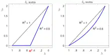
If an -norm is used to penalize deviations from zero given a single regressor, the solution path is given by
. Like , moves in the direction of the point when is close to zero; but unlike , the influence of diminishes in if increases (see figure).
Given multiple regressors, the moment that a parameter is activated (i.e. allowed to deviate from ) is also determined by a regressor's contribution to accuracy. First,
An of 75% means that in-sample accuracy improves by 75% if the unrestricted OLS solutions are used instead of the hypothesized values. The individual contribution of deviating from each hypothesis can be computed with the x matrix
where . If when is computed, then the diagonal elements of sum to . The diagonal values may be smaller than 0 or, less often, larger than 1. If regressors are uncorrelated, then the diagonal element of simply corresponds to the value between and .
A rescaled version of the adaptive lasso of can be obtained by setting .[8] If regressors are uncorrelated, the moment that the parameter is activated is given by the diagonal element of . Assuming for convenience that is a vector of zeros,
That is, if regressors are uncorrelated, again specifies the minimal influence of . Even when regressors are correlated, the first time that a regression parameter is activated occurs when is equal to the highest diagonal element of .
These results can be compared to a rescaled version of the lasso by defining , which is the average absolute deviation of from . Assuming that regressors are uncorrelated, then the moment of activation of the regressor is given by
For , the moment of activation is again given by . If is a vector of zeros and a subset of relevant parameters are equally responsible for a perfect fit of , then this subset is activated at a value of . The moment of activation of a relevant regressor then equals . In other words, the inclusion of irrelevant regressors delays the moment that relevant regressors are activated by this rescaled lasso. The adaptive lasso and the lasso are special cases of a '1ASTc' estimator. The latter only groups parameters together if the absolute correlation among regressors is larger than a user-specified value.[6]
Bayesian interpretation

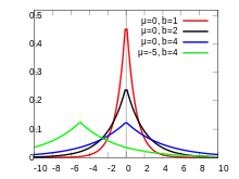
Just as ridge regression can be interpreted as linear regression for which the coefficients have been assigned normal prior distributions, lasso can be interpreted as linear regression for which the coefficients have Laplace prior distributions. The Laplace distribution is sharply peaked at zero (its first derivative is discontinuous at zero) and it concentrates its probability mass closer to zero than does the normal distribution. This provides an alternative explanation of why lasso tends to set some coefficients to zero, while ridge regression does not.[1]
Convex relaxation interpretation
Lasso can also be viewed as a convex relaxation of the best subset selection regression problem, which is to find the subset of covariates that results in the smallest value of the objective function for some fixed , where n is the total number of covariates. The " norm", , (the number of nonzero entries of a vector), is the limiting case of " norms", of the form (where the quotation marks signify that these are not really norms for since is not convex for , so the triangle inequality does not hold). Therefore, since p = 1 is the smallest value for which the " norm" is convex (and therefore actually a norm), lasso is, in some sense, the best convex approximation to the best subset selection problem, since the region defined by is the convex hull of the region defined by for .
参见
- 降维
- 特征选择
参考文献
- Tibshirani, Robert. 1996. “Regression Shrinkage and Selection via the lasso”. Journal of the Royal Statistical Society. Series B (methodological) 58 (1). Wiley: 267–88. http://www.jstor.org/stable/2346178 (页面存档备份,存于).
- Breiman, Leo. . Technometrics. 1995-11-01, 37 (4): 373–384 [2017-10-06]. ISSN 0040-1706. doi:10.2307/1269730. (原始内容存档于2020-06-08).
- Tibshirani, Robert. . Journal of the Royal Statistical Society. Series B (Methodological). 1996, 58 (1): 267–288 [2016-07-25]. (原始内容存档于2020-11-17).
- Tibshirani, Robert. . Statistics in Medicine. 1997-02-28, 16 (4): 385–395. ISSN 1097-0258. doi:10.1002/(sici)1097-0258(19970228)16:4%3C385::aid-sim380%3E3.0.co;2-3 (英语).
- Hoornweg, Victor. . . Hoornweg Press. 2018 [2023-08-08]. ISBN 978-90-829188-0-9. (原始内容存档于2023-11-02).
- Motamedi, Fahimeh; Sanchez, Horacio; Mehri, Alireza; Ghasemi, Fahimeh. . Bioinformatics. October 2021, 37 (19): 469–475. ISSN 1367-4803. PMID 34979024. doi:10.1093/bioinformatics/btab659.
- Zou, Hui. (PDF). 2006 [2023-08-08]. (原始内容存档 (PDF)于2021-07-11).
- Shaonan, Tian; Yu, Yan; Guo, Hui. . Journal of Banking & Finance. 2015, 52 (1): 89–100. doi:10.1016/j.jbankfin.2014.12.003
 .
. - Coad, Alex; Srhoj, Stjepan. . Small Business Economics. 2020, 55 (1): 541–565. doi:10.1007/s11187-019-00203-3
 .
.