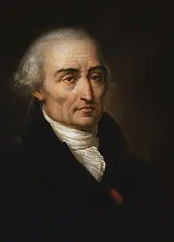
約瑟夫·拉格朗日 在分析力學裏,一个动力系统 的拉格朗日量 (英語:Lagrangian 拉格朗日函數 ,简称“拉氏量”,是描述整个物理系统的动力状态的函数 ,對於一般經典物理系統,通常定義為動能 減去勢能 [ 1]
L
=
T
−
V
{\displaystyle {\mathcal {L}}=T-V}
其中,
L
{\displaystyle {\mathcal {L}}}
T
{\displaystyle T}
V
{\displaystyle V}
在分析力学裡,假設已知一个系统的拉格朗日量,则可以将拉格朗日量直接代入拉格朗日方程式,稍加运算,即可求得此系统的运动方程式。
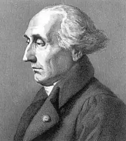
拉格朗日量是因數學家和天文學家約瑟夫·拉格朗日 而命名。
在场论,若
S
(
ϕ
)
=
∫
L
(
ϕ
(
x
)
,
∂
ϕ
(
x
)
,
x
)
d
n
x
{\displaystyle S(\phi )=\int {\mathcal {L}}(\phi (x),\partial \phi (x),x)d^{n}x}
是作用量,则拉格朗日方程是
δ
S
δ
ϕ
=
0
{\displaystyle {\frac {\delta S}{\delta \phi }}=0}
拉格朗日量是动能
T
{\displaystyle T}
V
{\displaystyle V}
L
=
T
−
V
{\displaystyle {\mathcal {L}}=T-V}
通常,動能的參數為廣義速度
q
˙
1
,
q
˙
2
,
q
˙
3
,
…
,
q
˙
N
{\displaystyle {\dot {q}}_{1},{\dot {q}}_{2},{\dot {q}}_{3},\dots ,{\dot {q}}_{N}}
t
{\displaystyle t}
q
1
,
q
2
,
q
3
,
…
,
q
N
;
t
{\displaystyle q_{1},q_{2},q_{3},\dots ,q_{N};t}
q
1
,
q
2
,
q
3
,
…
,
q
N
;
q
˙
1
,
q
˙
2
,
q
˙
3
,
…
,
q
˙
N
;
t
{\displaystyle q_{1},q_{2},q_{3},\dots ,q_{N};{\dot {q}}_{1},{\dot {q}}_{2},{\dot {q}}_{3},\dots ,{\dot {q}}_{N};t}
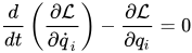
假設一個物理系統的拉格朗日量為
L
{\displaystyle {\mathcal {L}}}
d
d
t
(
∂
L
∂
q
˙
i
)
−
∂
L
∂
q
i
=
0
{\displaystyle {\frac {d}{dt}}\left({\frac {\partial {\mathcal {L}}}{\partial {\dot {q}}_{i}}}\right)-{\frac {\partial {\mathcal {L}}}{\partial q_{i}}}=0}
其中,
t
{\displaystyle t}
q
i
{\displaystyle q_{i}}
q
˙
i
{\displaystyle {\dot {q}}_{i}}
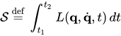
一個物理系統的作用量
S
{\displaystyle {\mathcal {S}}}
S
=
d
e
f
∫
t
1
t
2
L
(
q
,
q
˙
,
t
)
d
t
{\displaystyle {\mathcal {S}}\ {\stackrel {\mathrm {def} }{=}}\ \int _{t_{1}}^{t_{2}}L(\mathbf {q} ,{\dot {\mathbf {q} }},t)\,dt}
其中,
L
(
q
,
q
˙
,
t
)
{\displaystyle L(\mathbf {q} ,{\dot {\mathbf {q} }},t)}
q
=
(
q
1
,
q
2
,
…
,
q
N
)
{\displaystyle \mathbf {q} =\left(q_{1},q_{2},\ldots ,q_{N}\right)}
t
{\displaystyle t}
t
1
{\displaystyle t_{1}}
t
2
{\displaystyle t_{2}}
假若,作用量的一次變分
δ
S
=
0
{\displaystyle \delta {\mathcal {S}}=0}
S
{\displaystyle {\mathcal {S}}}
平穩值 ,則
q
(
t
)
{\displaystyle \mathbf {q} (t)}
詳盡相關導引,請參閱拉格朗日方程式。
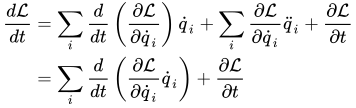
根据诺特定理,根据物理系统的对称性可以通过拉格朗日量导出守恒量。如果物理系统具有时间平移不变性则可以导出能量守恒 。导出过程如下,思考拉格朗日量對於時間的全導數:
d
L
d
t
=
∑
i
∂
L
∂
q
i
q
˙
i
+
∑
i
∂
L
∂
q
˙
i
q
¨
i
+
∂
L
∂
t
{\displaystyle {\frac {d{\mathcal {L}}}{dt}}=\sum _{i}{\frac {\partial {\mathcal {L}}}{\partial q_{i}}}{\dot {q}}_{i}+\sum _{i}{\frac {\partial {\mathcal {L}}}{\partial {\dot {q}}_{i}}}{\ddot {q}}_{i}+{\frac {\partial {\mathcal {L}}}{\partial t}}}
將拉格朗日方程式代入,可以得到
d
L
d
t
=
∑
i
d
d
t
(
∂
L
∂
q
˙
i
)
q
˙
i
+
∑
i
∂
L
∂
q
˙
i
q
¨
i
+
∂
L
∂
t
=
∑
i
d
d
t
(
∂
L
∂
q
˙
i
q
˙
i
)
+
∂
L
∂
t
{\displaystyle {\begin{aligned}{\frac {d{\mathcal {L}}}{dt}}&=\sum _{i}{\frac {d}{dt}}\left({\frac {\partial {\mathcal {L}}}{\partial {\dot {q}}_{i}}}\right){\dot {q}}_{i}+\sum _{i}{\frac {\partial {\mathcal {L}}}{\partial {\dot {q}}_{i}}}{\ddot {q}}_{i}+{\frac {\partial {\mathcal {L}}}{\partial t}}\\&=\sum _{i}{\frac {d}{dt}}\left({\frac {\partial {\mathcal {L}}}{\partial {\dot {q}}_{i}}}{\dot {q}}_{i}\right)+{\frac {\partial {\mathcal {L}}}{\partial t}}\\\end{aligned}}}
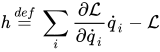
。 定義能量函數
h
(
q
1
,
q
2
,
q
3
,
…
;
q
˙
1
,
q
˙
2
,
q
˙
3
,
…
;
t
)
{\displaystyle {\mathit {h}}(q_{1},q_{2},q_{3},\dots ;{\dot {q}}_{1},{\dot {q}}_{2},{\dot {q}}_{3},\dots ;t)}
h
=
d
e
f
∑
i
∂
L
∂
q
˙
i
q
˙
i
−
L
{\displaystyle {\mathit {h}}\ {\stackrel {def}{=}}\ \sum _{i}{\frac {\partial {\mathcal {L}}}{\partial {\dot {q}}_{i}}}{\dot {q}}_{i}-{\mathcal {L}}}
則能量函數與拉格朗日量有以下含時關係式:
d
h
d
t
=
−
∂
L
∂
t
{\displaystyle {\frac {d{\mathit {h}}}{dt}}=-{\frac {\partial {\mathcal {L}}}{\partial t}}}
假若系统具有时间平移不变性,即拉格朗日量顯性地與時間無關,
∂
L
∂
t
=
0
{\displaystyle {\frac {\partial {\mathcal {L}}}{\partial t}}=0}
h
=
E
{\displaystyle {\mathit {h}}=E}
E
{\displaystyle E}
能量守恆 [ 2] 动量守恒 ,守恒量动量 为
∂
L
∂
q
˙
i
{\displaystyle {\frac {\partial {\mathcal {L}}}{\partial {\dot {q}}_{i}}}}
1941年杰西·道格拉斯指出,对于任意常微分方程组
F
i
(
t
,
q
j
,
q
j
′
,
q
j
″
)
=
0
{\displaystyle F_{i}(t,q_{j},q_{j}^{'},q_{j}^{''})=0}
S
=
∫
t
1
t
2
L
(
q
,
q
˙
,
t
)
d
t
{\displaystyle {\mathcal {S}}\ =\ \int _{t_{1}}^{t_{2}}L(\mathbf {q} ,{\dot {\mathbf {q} }},t)\,dt}
F
i
{\displaystyle F_{i}}
∂
F
i
∂
q
j
″
=
∂
F
j
∂
q
i
″
{\displaystyle {\frac {\partial F_{i}}{\partial q_{j}^{''}}}={\frac {\partial F_{j}}{\partial q_{i}^{''}}}}
∂
F
i
∂
q
j
−
∂
F
j
∂
q
i
=
1
2
d
d
t
(
∂
F
i
∂
q
j
′
−
∂
F
j
∂
q
i
′
)
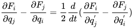
{\displaystyle {\frac {\partial F_{i}}{\partial q_{j}}}-{\frac {\partial F_{j}}{\partial q_{i}}}={\frac {1}{2}}{\frac {d}{dt}}({\frac {\partial F_{i}}{\partial q_{j}^{'}}}-{\frac {\partial F_{j}}{\partial q_{i}^{'}}})}
∂
F
i
∂
q
j
′
+
∂
F
j
∂
q
i
′
=
2
d
d
t
(
∂
F
j
∂
q
i
″
)
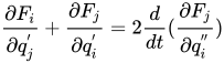
{\displaystyle {\frac {\partial F_{i}}{\partial q_{j}^{'}}}+{\frac {\partial F_{j}}{\partial q_{i}^{'}}}=2{\frac {d}{dt}}({\frac {\partial F_{j}}{\partial q_{i}^{''}}})}
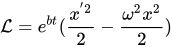
这一条件又称为亥姆霍兹条件。需要注意的是,这里
L
=
T
−
V
{\displaystyle {\mathcal {L}}=T-V}
L
{\displaystyle {\mathcal {L}}}
x
″
+
b
x
′
+
ω
2
x
=
0
{\displaystyle x^{''}+bx^{'}+\omega ^{2}x=0}
L
=
e
b
t
(
x
′
2
2
−
ω
2
x
2
2
)
{\displaystyle {\mathcal {L}}=e^{bt}({\frac {x^{'2}}{2}}-{\frac {\omega ^{2}x^{2}}{2}})}
[ 3]
拉格朗日表述是经典力学 的一种重新表述。拉格朗日表述的重要性,不只是因为它可以广泛应用在经典力学;而更是因为它能够帮助物理学家更深刻地了解一个物理系统的物理行为。雖然拉格朗日只是在尋找一種表述經典力學的方法,他用來推導拉格朗日方程式的平穩作用量原理 ,現在已被學術界公認為在量子力學 也極具功用。
拉格朗日表述不会被任何坐标系统捆绑住。拉格朗日表述使用广义坐标来描述系统的空间参数。它所涉及的物理量 是动能与势能,这些物理量的值不会随广义坐标的选择而改变。因此,對於系统的种种約束,可以选择一组最合适的广义坐标,来计算问题的解答。
拉格朗日表述能够简易地延伸至其他学术領域。电路学 、量子力学 、粒子物理学 、等等,都可以用拉格朗日表述来分析。
如果用同样的表述可以分析不同学术領域的物理系统,这些系统必定有結构上的类推。在一个学术領域的新发现,意味著很可能在另一个学术領域会有类似的现象。
拉格朗日量有一個優良的性質,那就是守恆定律 可以很容易地從它的表達式讀出來。例如,假設拉格朗日量
L
{\displaystyle {\mathcal {L}}}
q
˙
2
{\displaystyle {\dot {q}}_{2}}
q
2
{\displaystyle q_{2}}
p
2
{\displaystyle p_{2}}
L
(
q
1
,
q
3
,
q
4
,
…
;
q
˙
1
,
q
˙
2
,
q
˙
3
,
q
˙
4
,
…
;
t
)
{\displaystyle {\mathcal {L}}(q_{1},q_{3},q_{4},\dots ;{\dot {q}}_{1},{\dot {q}}_{2},{\dot {q}}_{3},{\dot {q}}_{4},\dots ;t)}
直接檢視,就可以發覺
L
{\displaystyle {\mathcal {L}}}
q
2
{\displaystyle q_{2}}
p
2
{\displaystyle p_{2}}
以此類推,假設,時間
t
{\displaystyle t}
L
{\displaystyle {\mathcal {L}}}
哈密頓量 守恆,即能量守恆。這種物理行為是諾特定理的一個特別案例。關於能量守恆問題,稍後會有更詳細解說。
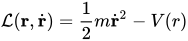
假设,在三维空间裏,一個運動中的粒子的動能為
T
=
1
2
m
r
˙
2
=
1
2
m
(
x
1
˙
2
+
x
2
˙
2
+
x
3
˙
2
)
{\displaystyle T={\frac {1}{2}}m{\dot {\mathbf {r} }}^{2}={\frac {1}{2}}m({\dot {x_{1}}}^{2}+{\dot {x_{2}}}^{2}+{\dot {x_{3}}}^{2})}
V
(
r
)
{\displaystyle V(r)}
L
(
r
,
r
˙
)
=
1
2
m
r
˙
2
−
V
(
r
)
{\displaystyle {\mathcal {L}}(\mathbf {r} ,{\dot {\mathbf {r} }})={\frac {1}{2}}m{\dot {\mathbf {r} }}^{2}-V(r)}
其中,
m
{\displaystyle m}
r
{\displaystyle \mathbf {r} }
v
{\displaystyle v}
採用直角坐标系 。那麼,拉格朗日方程式就是
d
d
t
(
∂
L
∂
x
˙
i
)
−
∂
L
∂
x
i
=
0
,
i
=
1
,
2
,
3
{\displaystyle {\frac {d}{dt}}\left({\frac {\partial {\mathcal {L}}}{\partial {\dot {x}}_{i}}}\right)-{\frac {\partial {\mathcal {L}}}{\partial x_{i}}}=0\ ,\qquad \qquad \qquad \qquad i=1,\ 2,\ 3}
其中,
x
i
{\displaystyle x_{i}}
r
{\displaystyle \mathbf {r} }
i
{\displaystyle i}
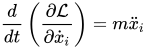
那麼,
d
d
t
(
∂
L
∂
x
˙
i
)
=
m
x
¨
i
{\displaystyle {\frac {d}{dt}}\left({\frac {\partial {\mathcal {L}}}{\partial {\dot {x}}_{i}}}\right)=m{\ddot {x}}_{i}}
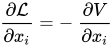
∂
L
∂
x
i
=
−
∂
V
∂
x
i
{\displaystyle {\frac {\partial {\mathcal {L}}}{\partial x_{i}}}=-\ {\frac {\partial V}{\partial x_{i}}}}
这物理系统的运动方程式为
m
r
¨
+
∇
V
=
0
{\displaystyle m{\ddot {\mathbf {r} }}+{\boldsymbol {\nabla }}V=0}
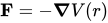
由於势能對於位置的負梯度是作用力:
F
=
−
∇
V
(
r
)
{\displaystyle \mathbf {F} =-{\boldsymbol {\nabla }}V(r)}
F
=
m
r
¨
{\displaystyle \mathbf {F} =m{\ddot {\mathbf {r} }}}
这方程式与牛顿第二定律 方程式完全相同。由此可以观察出,拉格朗日表述与牛顿表述的功能相等。
能量函數
h
{\displaystyle {\mathit {h}}}
h
=
∑
i
∂
L
∂
x
˙
i
x
˙
i
−
L
=
m
∑
i
x
˙
i
2
−
L
=
1
2
m
∑
i
x
˙
i
2
+
V
(
r
)
=
T
+
V
=
E
{\displaystyle {\mathit {h}}=\sum _{i}{\frac {\partial {\mathcal {L}}}{\partial {\dot {x}}_{i}}}{\dot {x}}_{i}-{\mathcal {L}}=m\sum _{i}{\dot {x}}_{i}^{2}-{\mathcal {L}}={\frac {1}{2}}m\sum _{i}{\dot {x}}_{i}^{2}+V(\mathbf {r} )=T+V=E}
由於拉格朗日量顯性地與時間無關,能量函數
h
{\displaystyle {\mathit {h}}}
E
{\displaystyle E}
假設選擇球坐标系 ,則拉格朗日量是
L
(
r
,
θ
,
φ
,
r
˙
,
θ
˙
,
φ
˙
)
=
m
2
(
r
˙
2
+
r
2
θ
˙
2
+
r
2
sin
2
θ
φ
˙
2
)
−
V
(
r
)
{\displaystyle {\mathcal {L}}(r,\ \theta ,\ \varphi ,\ {\dot {r}},\ {\dot {\theta }},\ {\dot {\varphi }})={\frac {m}{2}}({\dot {r}}^{2}+r^{2}{\dot {\theta }}^{2}+r^{2}\sin ^{2}\theta {\dot {\varphi }}^{2})-V(r)}
其中,
r
{\displaystyle r}
θ
{\displaystyle \theta }
天顶角 ,
φ
{\displaystyle \varphi }
方位角 。
稍加运算,得到运动方程式为:
d
d
t
(
∂
L
∂
r
˙
)
−
∂
L
∂
r
=
m
r
¨
−
m
r
(
θ
˙
2
+
sin
2
θ
φ
˙
2
)
+
d
V
d
r
=
0
{\displaystyle {\frac {d}{dt}}\left({\frac {\partial {\mathcal {L}}}{\partial {\dot {r}}}}\right)-{\frac {\partial {\mathcal {L}}}{\partial r}}=m{\ddot {r}}-mr({\dot {\theta }}^{2}+\sin ^{2}\theta {\dot {\varphi }}^{2})+{\frac {dV}{dr}}=0}
d
d
t
(
∂
L
∂
θ
˙
)
−
∂
L
∂
θ
=
d
d
t
(
m
r
2
θ
˙
)
−
m
r
2
sin
θ
cos
θ
φ
˙
2
=
0
{\displaystyle {\frac {d}{dt}}\left({\frac {\partial {\mathcal {L}}}{\partial {\dot {\theta }}}}\right)-{\frac {\partial {\mathcal {L}}}{\partial \theta }}={\frac {d}{dt}}(mr^{2}{\dot {\theta }})-mr^{2}\sin \theta \cos \theta {\dot {\varphi }}^{2}=0}
d
d
t
(
∂
L
∂
φ
˙
)
−
∂
L
∂
φ
=
d
d
t
(
m
r
2
sin
2
θ
φ
˙
)
=
0
{\displaystyle {\frac {d}{dt}}\left({\frac {\partial {\mathcal {L}}}{\partial {\dot {\varphi }}}}\right)-{\frac {\partial {\mathcal {L}}}{\partial \varphi }}={\frac {d}{dt}}(mr^{2}\sin ^{2}\theta {\dot {\varphi }})=0}
特別注意,
L
{\displaystyle {\mathcal {L}}}
φ
{\displaystyle \varphi }
φ
{\displaystyle \varphi }
L
z
=
m
r
2
sin
2
θ
φ
˙
{\displaystyle L_{z}=mr^{2}\sin ^{2}\theta {\dot {\varphi }}}
假定檢驗粒子的質量和電荷 超小,其對於外在系統的影響可以忽略。檢驗粒子時常可以想像為簡單的質點粒子,只擁有質量和電荷性質。像電子 或上夸克 一類的真實粒子具有更複雜的性質,它們的拉格朗日量含有更多項目。
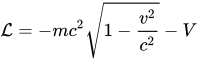
在狹義相對論 的四維空間 裏,一個移動中的粒子的相對論性拉格朗日量可以寫為[ 2]
L
=
−
m
c
2
1
−
v
2
c
2
−
V
{\displaystyle {\mathcal {L}}=-mc^{2}{\sqrt {1-{\frac {v^{2}}{c^{2}}}}}-V}
其中,
m
{\displaystyle m}
靜質量 ,
c
{\displaystyle c}
光速 ,
v
{\displaystyle v}
其拉格朗日方程式為
d
d
t
(
∂
L
∂
x
˙
i
)
−
∂
L
∂
x
i
=
d
d
t
(
γ
m
x
˙
i
)
+
∂
V
∂
x
i
=
0
{\displaystyle {\frac {d}{dt}}\left({\frac {\partial {\mathcal {L}}}{\partial {\dot {x}}_{i}}}\right)-{\frac {\partial {\mathcal {L}}}{\partial x_{i}}}={\frac {d}{dt}}(\gamma m{\dot {x}}_{i})+{\frac {\partial V}{\partial x_{i}}}=0}
其中,
γ
=
1
/
1
−
v
2
/
c
2
{\displaystyle \gamma =1/{\sqrt {1-v^{2}/c^{2}}}}
注意到動量
p
i
=
γ
m
x
˙
i
{\displaystyle p_{i}=\gamma m{\dot {x}}_{i}}
F
i
=
−
∂
V
∂
x
i
{\displaystyle F_{i}=-\ {\frac {\partial V}{\partial x_{i}}}}
F
=
d
p
d
t
{\displaystyle \mathbf {F} ={\frac {d\mathbf {p} }{dt}}}
因此,這拉格朗日量被認定為正確無誤。
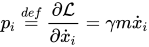
這粒子的廣義動量
p
i
{\displaystyle p_{i}}
p
i
=
d
e
f
∂
L
∂
x
˙
i
=
γ
m
x
˙
i
{\displaystyle p_{i}\ {\stackrel {def}{=}}\ {\frac {\partial {\mathcal {L}}}{\partial {\dot {x}}_{i}}}=\gamma m{\dot {x}}_{i}}
假設這物理系統的勢能為零,這粒子是自由粒子,則此系統的能量函數
h
{\displaystyle h}
h
=
∑
i
=
1
3
γ
m
x
˙
i
2
−
L
=
γ
m
v
2
+
m
c
2
1
−
v
2
c
2
=
γ
m
c
2
{\displaystyle h=\sum _{i=1}^{3}\gamma m{\dot {x}}_{i}^{2}-{\mathcal {L}}=\gamma mv^{2}+mc^{2}{\sqrt {1-{\frac {v^{2}}{c^{2}}}}}=\gamma mc^{2}}
這是質能方程式 :粒子的總能量等於其質量乘以光速平方 假設粒子速度遠小於光速,則拉格朗日量的動能部分可以近似為
−
m
c
2
1
−
v
2
c
2
≈
−
m
c
2
(
1
−
v
2
2
c
2
)
=
−
m
c
2
+
1
2
m
v
2
=
−
m
c
2
+
T
{\displaystyle -mc^{2}{\sqrt {1-{\frac {v^{2}}{c^{2}}}}}\approx -mc^{2}\left(1-{\frac {v^{2}}{2c^{2}}}\right)=-mc^{2}+{\frac {1}{2}}mv^{2}=-mc^{2}+T}
靜質量的能量
m
c
2
{\displaystyle mc^{2}}
變分 等於零)。相對論性拉格朗日量又變回經典拉格朗日量:
L
=
T
−
V
{\displaystyle {\mathcal {L}}=T-V}
一個移動於電磁場 的帶電粒子的相對論性拉格朗日量可以寫為
L
=
−
m
c
2
1
−
v
2
c
2
−
q
ϕ
(
r
)
+
q
v
⋅
A
(
r
,
t
)
{\displaystyle {\mathcal {L}}=-mc^{2}{\sqrt {1-{\frac {v^{2}}{c^{2}}}}}-q\phi (\mathbf {r} )+q\mathbf {v} \cdot \mathbf {A} (\mathbf {r} ,t)}
其中,
q
{\displaystyle q}
電荷量 ,
ϕ
{\displaystyle \phi }
電勢 ,
A
{\displaystyle \mathbf {A} }
其拉格朗日方程式為
d
d
t
(
∂
L
∂
x
˙
i
)
−
∂
L
∂
x
i
=
d
d
t
(
γ
m
x
˙
i
)
+
q
d
A
i
d
t
−
q
∂
ϕ
∂
x
i
−
q
∑
j
=
1
3
v
j
∂
A
j
∂
x
i
=
0
{\displaystyle {\frac {d}{dt}}\left({\frac {\partial {\mathcal {L}}}{\partial {\dot {x}}_{i}}}\right)-{\frac {\partial {\mathcal {L}}}{\partial x_{i}}}={\frac {d}{dt}}(\gamma m{\dot {x}}_{i})+q{\frac {dA_{i}}{dt}}-q{\frac {\partial \phi }{\partial x_{i}}}-q\sum _{j=1}^{3}v_{j}{\frac {\partial A_{j}}{\partial x_{i}}}=0}
所以,
d
d
t
(
γ
m
x
˙
i
)
=
−
q
d
A
i
d
t
+
q
∂
ϕ
∂
x
i
+
q
∑
j
=
1
3
v
j
∂
A
j
∂
x
i
{\displaystyle {\frac {d}{dt}}(\gamma m{\dot {x}}_{i})=-q{\frac {dA_{i}}{dt}}+q{\frac {\partial \phi }{\partial x_{i}}}+q\sum _{j=1}^{3}v_{j}{\frac {\partial A_{j}}{\partial x_{i}}}}
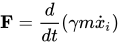
注意到作用力
F
=
d
d
t
(
γ
m
x
˙
i
)
{\displaystyle \mathbf {F} ={\frac {d}{dt}}(\gamma m{\dot {x}}_{i})}
電場
E
=
−
∇
ϕ
{\displaystyle \mathbf {E} =-\nabla \phi }
磁場
B
=
∇
×
A
{\displaystyle \mathbf {B} =\nabla \times \mathbf {A} }
勞侖茲力方程式 :
F
=
q
(
E
+
v
×
B
)
{\displaystyle \mathbf {F} =q(\mathbf {E} +\mathbf {v} \times \mathbf {B} )}
這拉格朗日量可以複製出勞侖茲力方程式。因此,這拉格朗日量被認定為正確無誤。
前面這些拉格朗日量都不具有協變形式,當變換坐標系 時,拉格朗日量的形式可能會有所改變。為了確保這形式不會改變,必須將拉格朗日量寫為協變形式。
對於自由粒子,作用量
A
{\displaystyle {\mathcal {A}}}
A
=
∫
t
1
t
2
L
d
t
=
∫
t
1
t
2
−
m
c
2
1
−
v
2
c
2
d
t
{\displaystyle {\mathcal {A}}=\int _{t_{1}}^{t_{2}}{\mathcal {L}}dt=\int _{t_{1}}^{t_{2}}-mc^{2}{\sqrt {1-{\frac {v^{2}}{c^{2}}}}}\ dt}
其中,
t
1
{\displaystyle t_{1}}
t
2
{\displaystyle t_{2}}
為了要使得拉格朗日量具有協變形式,必須引用張量 來表達。採用愛因斯坦求和約定 ,注意到四維速度與自己的內積:
U
α
U
α
=
γ
2
(
c
2
−
v
2
)
=
γ
2
c
2
(
1
−
v
2
c
2
)
{\displaystyle U^{\alpha }U_{\alpha }=\gamma ^{2}(c^{2}-v^{2})=\gamma ^{2}c^{2}\left(1-{\frac {v^{2}}{c^{2}}}\right)}
其中,
U
α
=
X
′
μ
=
d
X
α
d
τ
=
γ
(
c
,
v
1
,
v
2
,
v
3
)
{\displaystyle U^{\alpha }=X^{\prime \mu }={\frac {dX^{\alpha }}{d\tau }}=\gamma (c,v_{1},v_{2},v_{3})}
X
α
=
(
c
t
,
x
1
,
x
2
,
x
3
)
{\displaystyle X^{\alpha }=(ct,x_{1},x_{2},x_{3})}
τ
{\displaystyle \tau }
τ
{\displaystyle \tau }
將積分元素從微小時間元素
d
t
{\displaystyle dt}
d
τ
{\displaystyle d\tau }
d
t
=
γ
d
τ
{\displaystyle dt=\gamma d\tau }
A
=
∫
τ
1
τ
2
−
m
c
γ
U
α
U
α
γ
d
τ
=
∫
τ
1
τ
2
−
m
c
U
α
U
α
d
τ
{\displaystyle {\mathcal {A}}=\int _{\tau _{1}}^{\tau _{2}}-{\frac {mc}{\gamma }}{\sqrt {U^{\alpha }U_{\alpha }}}\ \gamma d\tau =\int _{\tau _{1}}^{\tau _{2}}-mc{\sqrt {U^{\alpha }U_{\alpha }}}\ d\tau }
協變的拉格朗日量
L
¯
{\displaystyle {\bar {\mathcal {L}}}}
[ 2]
L
¯
=
γ
L
=
−
m
c
U
α
U
α
=
−
m
c
g
α
β
U
α
U
β
{\displaystyle {\bar {\mathcal {L}}}=\gamma {\mathcal {L}}=-mc{\sqrt {U^{\alpha }U_{\alpha }}}=-mc{\sqrt {g_{\alpha \beta }U^{\alpha }U^{\beta }}}}
其中,
g
α
β
{\displaystyle g_{\alpha \beta }}
閔可夫斯基度規 。
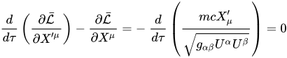
其拉格朗日方程式為
d
d
τ
(
∂
L
¯
∂
X
′
μ
)
−
∂
L
¯
∂
X
μ
=
−
d
d
τ
(
m
c
X
μ
′
g
α
β
U
α
U
β
)
=
0
{\displaystyle {\frac {d}{d\tau }}\left({\frac {\partial {\bar {\mathcal {L}}}}{\partial {X}^{\prime \mu }}}\right)-{\frac {\partial {\bar {\mathcal {L}}}}{\partial X^{\mu }}}=-\ {\frac {d}{d\tau }}\left({\frac {mc{X}_{\mu }^{\prime }}{\sqrt {g_{\alpha \beta }U^{\alpha }U^{\beta }}}}\right)=0}
注意到約束
U
α
U
α
=
γ
2
(
c
2
−
v
2
)
=
c
2
{\displaystyle U^{\alpha }U_{\alpha }=\gamma ^{2}(c^{2}-v^{2})=c^{2}}
d
d
τ
(
m
X
μ
′
)
=
m
X
μ
′
′
=
0
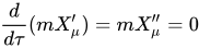
{\displaystyle {\frac {d}{d\tau }}(m{X}_{\mu }^{\prime })=m{X}_{\mu }^{\prime \prime }=0}
現在假設這粒子是移動於電磁場的帶電粒子。電磁場的協變位勢可以寫為
q
ϕ
(
r
)
−
q
v
⋅
A
(
r
,
t
)
=
q
U
α
A
α
(
X
β
)
/
γ
{\displaystyle q\phi (\mathbf {r} )-q\mathbf {v} \cdot \mathbf {A} (\mathbf {r} ,t)=qU^{\alpha }\mathbb {A} _{\alpha }(X^{\beta })/\gamma }
其中,
A
α
=
(
ϕ
/
c
,
−
A
1
,
−
A
2
,
−
A
3
)
{\displaystyle \mathbb {A} _{\alpha }=(\phi /c,-A_{1},-A_{2},-A_{3})}
協變的拉格朗日量
L
¯
{\displaystyle {\bar {\mathcal {L}}}}
[ 2]
L
¯
=
γ
L
=
−
m
c
g
α
β
U
α
U
β
−
q
U
α
A
α
(
X
β
)
{\displaystyle {\bar {\mathcal {L}}}=\gamma {\mathcal {L}}=-mc{\sqrt {g_{\alpha \beta }U^{\alpha }U^{\beta }}}-qU^{\alpha }\mathbb {A} _{\alpha }(X^{\beta })}
其拉格朗日方程式為
d
d
τ
(
∂
L
¯
∂
X
′
μ
)
−
∂
L
¯
∂
X
μ
=
−
d
d
τ
(
m
X
μ
′
+
q
A
μ
)
+
q
U
α
∂
A
α
∂
X
μ
=
0
{\displaystyle {\frac {d}{d\tau }}\left({\frac {\partial {\bar {\mathcal {L}}}}{\partial {X}^{\prime \mu }}}\right)-{\frac {\partial {\bar {\mathcal {L}}}}{\partial X^{\mu }}}=-{\frac {d}{d\tau }}(m{X}_{\mu }^{\prime }+q\mathbb {A} _{\mu })+qU^{\alpha }{\frac {\partial \mathbb {A} _{\alpha }}{\partial X^{\mu }}}=0}
經過一番運算,可以得到
m
X
μ
′
′
=
−
q
d
d
τ
(
A
μ
)
+
q
U
α
∂
A
α
∂
X
μ
=
−
q
d
X
α
d
τ
∂
(
A
μ
)
∂
X
α
+
q
U
α
∂
A
α
∂
X
μ
=
q
U
α
(
∂
A
α
∂
X
μ
−
∂
(
A
μ
)
∂
X
α
)
=
q
U
α
F
μ
α
{\displaystyle {\begin{aligned}m{X}_{\mu }^{\prime \prime }&=-q{\frac {d}{d\tau }}(\mathbb {A} _{\mu })+qU^{\alpha }{\frac {\partial \mathbb {A} _{\alpha }}{\partial X^{\mu }}}\\&=-q{\frac {dX^{\alpha }}{d\tau }}{\frac {\partial (\mathbb {A} _{\mu })}{\partial X^{\alpha }}}+qU^{\alpha }{\frac {\partial \mathbb {A} _{\alpha }}{\partial X^{\mu }}}\\&=qU^{\alpha }\left({\frac {\partial \mathbb {A} _{\alpha }}{\partial X^{\mu }}}-{\frac {\partial (\mathbb {A} _{\mu })}{\partial X^{\alpha }}}\right)\\&=qU^{\alpha }F_{\mu \alpha }\\\end{aligned}}}
其中,
F
μ
α
{\displaystyle F_{\mu \alpha }}
這正是勞侖茲力方程式的協變形式。總結,協變的拉格朗日方程式可以複製出協變的勞侖茲力方程式。
S
[
A
]
=
∫
M
(
−
1
2
F
∧
⋆
F
+
A
∧
⋆
J
)
{\displaystyle {\mathcal {S}}[\mathbf {A} ]=\int _{\mathcal {M}}\left(-{\frac {1}{2}}\,\mathbf {F} \wedge \star \mathbf {F} +\mathbf {A} \wedge \star \mathbf {J} \right)}
d
⋆
F
=
J
{\displaystyle \mathrm {d} {\star }\mathbf {F} =\mathbf {J} }
d
F
=
0
{\displaystyle \mathrm {d} \mathbf {F} =0}
L
Q
E
D
=
i
ℏ
c
ψ
¯
D
/
ψ
−
m
c
2
ψ
¯
ψ
−
1
4
μ
0
F
μ
ν
F
μ
ν
{\displaystyle {\mathcal {L}}_{\mathrm {QED} }=i\hbar c{\bar {\psi }}{D}\!\!\!\!/\ \psi -mc^{2}{\bar {\psi }}\psi -{1 \over 4\mu _{0}}F_{\mu \nu }F^{\mu \nu }}
L
Q
C
D
=
∑
n
(
i
ℏ
c
ψ
¯
n
D
/
ψ
n
−
m
n
c
2
ψ
¯
n
ψ
n
)
−
1
4
G
α
μ
ν
G
α
μ
ν
{\displaystyle {\mathcal {L}}_{\mathrm {QCD} }=\sum _{n}\left(i\hbar c{\bar {\psi }}_{n}{D}\!\!\!\!/\ \psi _{n}-m_{n}c^{2}{\bar {\psi }}_{n}\psi _{n}\right)-{1 \over 4}G^{\alpha }{}_{\mu \nu }G_{\alpha }{}^{\mu \nu }}
包括QED、量子色动力学 、等
广义相对论 中拉格朗日量密度为:
L
GR
=
L
EH
+
L
matter
=
c
4
16
π
G
(
R
−
2
Λ
)
+
L
matter
{\displaystyle {\mathcal {L}}_{\text{GR}}={\mathcal {L}}_{\text{EH}}+{\mathcal {L}}_{\text{matter}}={\frac {c^{4}}{16\pi G}}\left(R-2\Lambda \right)+{\mathcal {L}}_{\text{matter}}}
其中,
Λ
{\displaystyle \Lambda }
宇宙学常数 ,
R
{\displaystyle R}
度规张量 的缩并。
L
E
H
{\displaystyle L_{EH}}
李群 的纤维丛上表现得很好后得到的结果。通过加入对称群
S
O
(
3
,
1
)
{\displaystyle SO(3,1)}
[ 4] [ 5]
通过对
g
μ
ν
{\displaystyle g_{\mu \nu }}
R
μ
ν
−
1
2
R
g
μ
ν
+
g
μ
ν
Λ
=
8
π
G
c
4
T
μ
ν
{\displaystyle R_{\mu \nu }-{\frac {1}{2}}Rg_{\mu \nu }+g_{\mu \nu }\Lambda ={\frac {8\pi G}{c^{4}}}T_{\mu \nu }}
这也被称为爱因斯坦场方程。
T
μ
ν
{\displaystyle T_{\mu \nu }}
T
μ
ν
≡
−
2
−
g
δ
(
L
m
a
t
t
e
r
−
g
)
δ
g
μ
ν
=
−
2
δ
L
m
a
t
t
e
r
δ
g
μ
ν
+
g
μ
ν
L
m
a
t
t
e
r
{\displaystyle T_{\mu \nu }\equiv {\frac {-2}{\sqrt {-g}}}{\frac {\delta ({\mathcal {L}}_{\mathrm {matter} }{\sqrt {-g}})}{\delta g^{\mu \nu }}}=-2{\frac {\delta {\mathcal {L}}_{\mathrm {matter} }}{\delta g^{\mu \nu }}}+g_{\mu \nu }{\mathcal {L}}_{\mathrm {matter} }}
其中,
g
{\displaystyle g}
度规张量 的行列式 。在广义相对论中,拉格朗日密度积分时的提及元变为
−
g
d
4
x
{\displaystyle {\sqrt {-g}}d^{4}x}
雅可比行列式 。负号是为了使根号下为正。
在广义相对论下,包含爱因斯坦-希尔伯特作用量电磁场的拉格朗日密度为:
L
(
x
)
=
j
μ
(
x
)
A
μ
(
x
)
−
1
4
μ
0
F
μ
ν
(
x
)
F
ρ
σ
(
x
)
g
μ
ρ
(
x
)
g
ν
σ
(
x
)
+
c
4
16
π
G
R
(
x
)
=
L
Maxwell
+
L
Einstein-Hilbert
{\displaystyle {\begin{aligned}{\mathcal {L}}(x)&=j^{\mu }(x)A_{\mu }(x)-{1 \over 4\mu _{0}}F_{\mu \nu }(x)F_{\rho \sigma }(x)g^{\mu \rho }(x)g^{\nu \sigma }(x)+{\frac {c^{4}}{16\pi G}}R(x)\\&={\mathcal {L}}_{\text{Maxwell}}+{\mathcal {L}}_{\text{Einstein-Hilbert}}\end{aligned}}}
L
m
a
t
t
e
r
{\displaystyle {\mathcal {L}}_{matter}}
g
μ
ν
(
x
)
{\displaystyle g_{\mu \nu }(x)}
闵氏时空 拉格朗日量中的闵可夫斯基矩阵可以简单得到这个形式。我们可以得到在电磁场中的爱因斯坦场方程。能动张量为:
T
μ
ν
(
x
)
=
2
−
g
(
x
)
δ
δ
g
μ
ν
(
x
)
S
Maxwell
=
1
μ
0
(
F
λ
μ
(
x
)
F
ν
λ
(
x
)
−
1
4
g
μ
ν
(
x
)
F
ρ
σ
(
x
)
F
ρ
σ
(
x
)
)
{\displaystyle T^{\mu \nu }(x)={\frac {2}{\sqrt {-g(x)}}}{\frac {\delta }{\delta g_{\mu \nu }(x)}}{\mathcal {S}}_{\text{Maxwell}}={\frac {1}{\mu _{0}}}\left(F_{{\text{ }}\lambda }^{\mu }(x)F^{\nu \lambda }(x)-{\frac {1}{4}}g^{\mu \nu }(x)F_{\rho \sigma }(x)F^{\rho \sigma }(x)\right)}
T
=
g
μ
ν
T
μ
ν
=
0
{\displaystyle T=g_{\mu \nu }T^{\mu \nu }=0}
如果同时对爱因斯坦场方程 两边同时缩并:
R
=
−
8
π
G
c
4
T
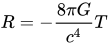
{\displaystyle R=-{\frac {8\pi G}{c^{4}}}T}
这意味着曲率张量也是无迹的,方程可以化简为:
R
μ
ν
=
8
π
G
c
4
1
μ
0
(
F
λ
μ
(
x
)
F
ν
λ
(
x
)
−
1
4
g
μ
ν
(
x
)
F
ρ
σ
(
x
)
F
ρ
σ
(
x
)
)
{\displaystyle R^{\mu \nu }={\frac {8\pi G}{c^{4}}}{\frac {1}{\mu _{0}}}\left(F_{{\text{ }}\lambda }^{\mu }(x)F^{\nu \lambda }(x)-{\frac {1}{4}}g^{\mu \nu }(x)F_{\rho \sigma }(x)F^{\rho \sigma }(x)\right)}
另外,弯曲时空的麦克斯韦方程组 为:
D
μ
F
μ
ν
=
−
μ
0
j
ν
{\displaystyle D_{\mu }F^{\mu \nu }=-\mu _{0}j^{\nu }}
其中,
D
μ
{\displaystyle D_{\mu }}
j
μ
=
0
{\displaystyle j^{\mu }=0}
Q
{\displaystyle Q}
d
s
2
=
(
1
−
2
M
r
+
Q
2
r
2
)
d
t
2
−
(
1
−
2
M
r
+
Q
2
r
2
)
−
1
d
r
2
−
r
2
d
Ω
2
{\displaystyle ds^{2}=\left(1-{\frac {2M}{r}}+{\frac {Q^{2}}{r^{2}}}\right)dt^{2}-\left(1-{\frac {2M}{r}}+{\frac {Q^{2}}{r^{2}}}\right)^{-1}dr^{2}-r^{2}d\Omega ^{2}}
一个可能的统一电磁场和引力场的理论是卡鲁扎-克莱因理论。[ 4]
^ Torby, Bruce. Advanced Dynamics for Engineers . HRW Series in Mechanical Engineering. United States of America: CBS College Publishing. 1984. ISBN 0-03-063366-4 (英语) . ^ 2.0 2.1 2.2 2.3 Goldstein, Herbert , Classical Mechanics 3rd, United States of America: Addison Wesley: pp. 61, 312–324, 1980, ISBN 0201657023 (英语) ^ Kushagra Nigam; Kinjal Banerjee. A Brief Review of Helmholtz Conditions . arxiv. 2016. ^ 4.0 4.1 David Bleecker, (1981) "Gauge Theory and Variational Principles" Addison-Wesley
^ Jurgen Jost, (1995) "Riemannian Geometry and Geometric Analysis", Springer
拉格朗日乘数 拉格朗日插值法
拉格朗日四平方和定理
拉格朗日定理 (群論) 拉格朗日定理 (數論)
拉格朗日恒等式
拉格朗日恒等式 (邊值問題) 拉格朗日三角恆等式 拉格朗日力学 拉格朗日中值定理
拉格朗日穩定性 拉格朗日方程
拉格朗日量 拉格朗日分析 拉格朗日和欧拉流场规范 拉格朗日拟序结构
拉格朗日点 拉格朗日格拉斯曼流形 拉格朗日括号
拉格朗日鬆弛 拉格朗日對偶
拉格朗日密度
拉格朗日不變量
拉格朗日子流形
拉格朗日系统 欧拉-拉格朗日方程