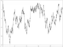
A Brownian bridge is a continuous-time stochastic process B(t) whose probability distribution is the conditional probability distribution of a standard Wiener process W(t) (a mathematical model of Brownian motion) subject to the condition (when standardized) that W(T) = 0, so that the process is pinned to the same value at both t = 0 and t = T. More precisely:
The expected value of the bridge at any t in the interval [0,T] is zero, with variance , implying that the most uncertainty is in the middle of the bridge, with zero uncertainty at the nodes. The covariance of B(s) and B(t) is , or s(T − t)/T if s < t. The increments in a Brownian bridge are not independent.
Relation to other stochastic processes
If W(t) is a standard Wiener process (i.e., for t ≥ 0, W(t) is normally distributed with expected value 0 and variance t, and the increments are stationary and independent), then
is a Brownian bridge for t ∈ [0, T]. It is independent of W(T)[1]
Conversely, if B(t) is a Brownian bridge and Z is a standard normal random variable independent of B, then the process
is a Wiener process for t ∈ [0, 1]. More generally, a Wiener process W(t) for t ∈ [0, T] can be decomposed into
Another representation of the Brownian bridge based on the Brownian motion is, for t ∈ [0, T]
Conversely, for t ∈ [0, ∞]
The Brownian bridge may also be represented as a Fourier series with stochastic coefficients, as
where are independent identically distributed standard normal random variables (see the Karhunen–Loève theorem).
A Brownian bridge is the result of Donsker's theorem in the area of empirical processes. It is also used in the Kolmogorov–Smirnov test in the area of statistical inference.
Intuitive remarks
A standard Wiener process satisfies W(0) = 0 and is therefore "tied down" to the origin, but other points are not restricted. In a Brownian bridge process on the other hand, not only is B(0) = 0 but we also require that B(T) = 0, that is the process is "tied down" at t = T as well. Just as a literal bridge is supported by pylons at both ends, a Brownian Bridge is required to satisfy conditions at both ends of the interval [0,T]. (In a slight generalization, one sometimes requires B(t1) = a and B(t2) = b where t1, t2, a and b are known constants.)
Suppose we have generated a number of points W(0), W(1), W(2), W(3), etc. of a Wiener process path by computer simulation. It is now desired to fill in additional points in the interval [0,T], that is to interpolate between the already generated points W(0) and W(T). The solution is to use a Brownian bridge that is required to go through the values W(0) and W(T).
General case
For the general case when B(t1) = a and B(t2) = b, the distribution of B at time t ∈ (t1, t2) is normal, with mean
and variance
and the covariance between B(s) and B(t), with s < t is
References
- ↑ Aspects of Brownian motion, Springer, 2008, R. Mansuy, M. Yor page 2