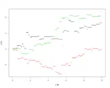
In the theory of stochastic processes, a part of the mathematical theory of probability, the variance gamma (VG) process, also known as Laplace motion, is a Lévy process determined by a random time change. The process has finite moments, distinguishing it from many Lévy processes. There is no diffusion component in the VG process and it is thus a pure jump process. The increments are independent and follow a variance-gamma distribution, which is a generalization of the Laplace distribution.
There are several representations of the VG process that relate it to other processes. It can for example be written as a Brownian motion with drift subjected to a random time change which follows a gamma process (equivalently one finds in literature the notation ):
An alternative way of stating this is that the variance gamma process is a Brownian motion subordinated to a gamma subordinator.
Since the VG process is of finite variation it can be written as the difference of two independent gamma processes:[1]
where
Alternatively it can be approximated by a compound Poisson process that leads to a representation with explicitly given (independent) jumps and their locations. This last characterization gives an understanding of the structure of the sample path with location and sizes of jumps.[2]
On the early history of the variance-gamma process see Seneta (2000).[3]
Moments
The mean of a variance gamma process is independent of and and is given by
The variance is given as
The 3rd central moment is
The 4th central moment is
Option pricing
The VG process can be advantageous to use when pricing options since it allows for a wider modeling of skewness and kurtosis than the Brownian motion does. As such the variance gamma model allows to consistently price options with different strikes and maturities using a single set of parameters. Madan and Seneta present a symmetric version of the variance gamma process.[4] Madan, Carr and Chang [1] extend the model to allow for an asymmetric form and present a formula to price European options under the variance gamma process.
Hirsa and Madan show how to price American options under variance gamma.[5] Fiorani presents numerical solutions for European and American barrier options under variance gamma process.[6] He also provides computer code to price vanilla and barrier European and American barrier options under variance gamma process.
Lemmens et al.[7] construct bounds for arithmetic Asian options for several Lévy models including the variance gamma model.
Applications to credit risk modeling
The variance gamma process has been successfully applied in the modeling of credit risk in structural models. The pure jump nature of the process and the possibility to control skewness and kurtosis of the distribution allow the model to price correctly the risk of default of securities having a short maturity, something that is generally not possible with structural models in which the underlying assets follow a Brownian motion. Fiorani, Luciano and Semeraro[8] model credit default swaps under variance gamma. In an extensive empirical test they show the overperformance of the pricing under variance gamma, compared to alternative models presented in literature.
Simulation
Monte Carlo methods for the variance gamma process are described by Fu (2000).[9] Algorithms are presented by Korn et al. (2010).[10]
Simulating VG as gamma time-changed Brownian motion
- Input: VG parameters and time increments , where
- Initialization: Set X(0) = 0.
- Loop: For i = 1 to N:
- Generate independent gamma , and normal variates, independently of past random variates.
- Return
Simulating VG as difference of gammas
This approach[9][10] is based on the difference of gamma representation , where are defined as above.
- Input: VG parameters ] and time increments , where
- Initialization: Set X(0) = 0.
- Loop: For i = 1 to N:
- Generate independent gamma variates independently of past random variates.
- Return
Variance gamma as 2-EPT distribution
Under the restriction that is integer the variance gamma distribution can be represented as a 2-EPT probability density function. Under this assumption it is possible to derive closed form vanilla option prices and their associated Greeks. For a comprehensive description see.[11]
References
- 1 2 Dilip Madan; Peter Carr; Eric Chang (1998). "The Variance Gamma Process and Option Pricing" (PDF). European FinanceReview. 2: 79–105.
- ↑ Kotz, Samuel; Kozubowski, Tomasz J.; Podgórski, Krzysztof (2001). The Laplace distribution and generalizations : a revisit with applications to communications, economics, engineering, and finance. Boston [u.a.]: Birkhäuser. ISBN 978-0817641665.
- ↑ Eugene Seneta (2000). "The Early Years of the Variance–Gamma Process". In Michael C. Fu; Robert A. Jarrow; Ju-Yi J. Yen; Robert J. Elliott (eds.). Advances in Mathematical Finance. Boston: Birkhauser. ISBN 978-0-8176-4544-1.
- ↑ Madan, Dilip B.; Seneta, Eugene (1990). "The Variance Gamma (V.G.) Model for Share Market Returns". Journal of Business. 63 (4): 511–524. doi:10.1086/296519. JSTOR 2353303.
- ↑ Hirsa, Ali; Madan, Dilip B. (2003). "Pricing American Options Under Variance Gamma". Journal of Computational Finance. 7 (2): 63–80. doi:10.21314/JCF.2003.112. S2CID 8283519.
- ↑ Filo Fiorani (2004). Option Pricing Under the Variance Gamma Process. Unpublished dissertation. p. 380. SSRN 1411741. PDF.
- ↑ Lemmens, Damiaan; Liang, Ling Zhi; Tempere, Jacques; De Schepper, Ann (2010), "Pricing bounds for discrete arithmetic Asian options under Lévy models", Physica A: Statistical Mechanics and Its Applications, 389 (22): 5193–5207, Bibcode:2010PhyA..389.5193L, doi:10.1016/j.physa.2010.07.026
- ↑ Filo Fiorani, Elisa Luciano and Patrizia Semeraro, (2007), Single and Joint Default in a Structural Model with Purely Discontinuous Assets, Working Paper No. 41, Carlo Alberto Notebooks, Collegio Carlo Alberto. URL PDF
- 1 2 Michael C. Fu (2000). "Variance-Gamma and Monte Carlo". In Michael C. Fu; Robert A. Jarrow; Ju-Yi J. Yen; Robert J. Elliott (eds.). Advances in Mathematical Finance. Boston: Birkhauser. ISBN 978-0-8176-4544-1.
- 1 2 Ralf Korn; Elke Korn & Gerald Kroisandt (2010). Monte Carlo Methods and Models in Finance and Insurance. Boca Raton, Fla.: Chapman and Hall/CRC. ISBN 978-1-4200-7618-9. (Section 7.3.3)
- ↑ Sexton, C. and Hanzon,B.,"State Space Calculations for two-sided EPT Densities with Financial Modelling Applications", www.2-ept.com