Forward model

The centerpiece of seismic linear inversion is the forward model which models the generation of the experimental data collected.^[1] According to Wiggins (1972),^[4] it provides a functional (computational) relationship between the model parameters and calculated values for the observed traces. Depending on the seismic data collected, this model may vary from the classical wave equations for predicting particle displacement or fluid pressure for sound wave propagation through rock or fluids, to some variants of these classical equations. For example, the forward model in Tarantola (1984)^[5] is the wave equation for pressure variation in a liquid media during seismic wave propagation while by assuming constant velocity layers with plane interfaces, Kanasewich and Chiu (1985)^[6] used the brachistotrone model of John Bernoulli for travel time of a ray along a path. In Cooke and Schneider (1983),^[1] the model is a synthetic trace generation algorithm expressed as in Eqn. 3, where R(t) is generated in the Z-domain by recursive formula. In whatever form the forward model appears, it is important that it not only predicts the collected field data, but also models how the data is generated. Thus, the forward model by Cooke and Schneider (1983)^[1] can only be used to invert CMP data since the model invariably assumes no spreading loss by mimicking the response of a laterally homogeneous earth to a plane-wave source

1. ${\displaystyle t=\sum _{i=1}^{n}{\frac {{\big [}(x_{i}-x_{i-1})^{2}+(y_{i}-y_{i-1})^{2}+(z_{i}-z_{i-1})^{2}{\big ]}^{\frac {1}{2}}}{v_{i}}}}$
where t is ray travel time, x, y, z are depth coordinates and vi is the constant velocity between interfaces i − 1 and i.
2. ${\displaystyle \left[{\frac {1}{K({\vec {r}})}}{\frac {\partial ^{2}}{\partial t^{2}}}-\nabla \cdot {\big (}{\frac {1}{\rho ({\vec {r}}{\big )}}}\nabla )\right]U({\vec {r}},t)=s({\vec {r}},t)}$
where ${\displaystyle K({\vec {r}})}$ represent bulk modulus, ${\displaystyle \rho ({\vec {r}})}$ density, ${\displaystyle s({\vec {r}},t)}$ the source of acoustic waves, and ${\displaystyle U({\vec {r}},t)}$ the pressure variation.
3. ${\displaystyle s(t)=w(t)*R(t)}$

where s(t) = synthetic trace, w(t) = source wavelet, and R(t) = reflectivity function.

Objective function

An important numerical process in inverse modeling is to minimize the objective function, which is a function defined in terms of the difference between the collected field seismic data and the numerically computed seismic data. Classical objective functions include the sum of squared deviations between experimental and numerical data, as in the least squares methods, the sum of the magnitude of the difference between field and numerical data, or some variant of these definitions. Irrespective of the definition used, numerical solution of the inverse problem is obtained as earth model that minimize the objective function.

In addition to the objective function, other constraints like known model parameters and known layer interfaces in some regions of the earth are also incorporated in the inverse modeling procedure. These constraints, according to Francis 2006,^[3] help to reduce non-uniqueness of the inversion solution by providing a priori information that is not contained in the inverted data while Cooke and Schneider (1983)^[1] reports their useful in controlling noise and when working in a geophysically well-known area.

Mathematical analysis of generalized linear inversion procedure

The objective of mathematical analysis of inverse modeling is to cast the generalized linear inverse problem into a simple matrix algebra by considering all the components described in previous sections. viz; forward model, objective function etc. Generally, the numerically generated seismic data are non-linear functions of the earth model parameters. To remove the non-linearity and create a platform for application of linear algebra concepts, the forward model is linearized by expansion using a Taylor series as carried out below. For more details see Wiggins (1972),^[4] Cooke and Schneider (1983).^[1]

Consider a set of ${\displaystyle m}$ seismic field observations ${\displaystyle F_{j}}$, for ${\displaystyle j=1,\ldots ,m}$ and a set of ${\displaystyle n}$ earth model parameters ${\displaystyle p_{i}}$ to be inverted for, for ${\displaystyle i=1,\ldots ,n}$. The field observations can be represented in either ${\displaystyle {\vec {F}}\,({\vec {p}})}$ or ${\displaystyle F_{j}\,(p_{i})}$, where ${\displaystyle {\vec {p}}}$ and ${\displaystyle {\vec {F}}\,({\vec {p}})}$ are vectorial representations of model parameters and the field observations as a function of earth parameters. Similarly, for ${\displaystyle q_{i}}$ representing guesses of model parameters, ${\displaystyle {\vec {F}}\,({\vec {q}})}$ is the vector of numerical computed seismic data using the forward model of Sec. 1.3. Taylor's series expansion of ${\displaystyle {\vec {F}}\,({\vec {p}})}$ about ${\displaystyle {\vec {q}}}$ is given below.

4. ${\displaystyle {\vec {F}}\,({\vec {p}})={\vec {F}}\,({\vec {q}})+({\vec {p}}-{\vec {q}}){\frac {\partial {\vec {F}}\,({\vec {q}})}{\partial {\vec {p}}}}+({\vec {p}}-{\vec {q}})^{2}{\frac {\partial ^{2}{\vec {F}}\,({\vec {q}})}{\partial {\vec {p}}^{2}}}+O({\vec {p}}-{\vec {q}})^{3}}$
On linearization by dropping the non-linear terms (terms with (p⃗ − ⃗q) of order 2 and above), the equation becomes
5. ${\displaystyle {\vec {F}}\,({\vec {p}})-{\vec {F}}\,({\vec {q}})=({\vec {p}}-{\vec {q}}){\frac {\partial {\vec {F}}\,({\vec {q}})}{\partial {\vec {p}}}}}$
Considering that ${\displaystyle {\vec {F}}}$ has ${\displaystyle m}$ components and ${\displaystyle {\vec {p}}}$ and ${\displaystyle {\vec {q}}}$ have ${\displaystyle n}$ components, the discrete form of Eqn. 5 results in a system of ${\displaystyle m}$ linear equations in ${\displaystyle n}$ variables whose matrix form is shown below.
6. ${\displaystyle \Delta {\vec {F}}=\mathbf {A} \,\Delta {\vec {p}}}$
7. ${\displaystyle \Delta {\vec {F}}={\begin{bmatrix}F_{1}({\vec {p}})-F_{1}({\vec {q}})\\\vdots \\F_{m}({\vec {p}})-F_{m}({\vec {q}})\end{bmatrix}}}$
8. ${\displaystyle \Delta {\vec {p}}={\vec {p}}-{\vec {q}}={\begin{bmatrix}p_{1}-q_{1}\\\vdots \\p_{n}-q_{n}\end{bmatrix}}}$
9. ${\displaystyle \mathbf {A} ={\begin{bmatrix}{\frac {\partial F_{1}({\vec {q}})}{\partial p_{1}}}&{\frac {\partial F_{1}({\vec {q}})}{\partial p_{2}}}&\cdots &{\frac {\partial F_{1}({\vec {q}})}{\partial p_{n}}}\\{\frac {\partial F_{2}({\vec {q}})}{\partial p_{1}}}&\cdots &{\frac {\partial F_{2}({\vec {q}})}{\partial p_{n-1}}}&{\frac {\partial F_{2}({\vec {q}})}{\partial p_{n}}}\\\vdots &{\frac {\partial F_{j}({\vec {q}})}{\partial p_{i}}}&\vdots &\vdots \\{\frac {\partial F_{m}({\vec {q}})}{\partial p_{1}}}&{\frac {\partial F_{m}({\vec {q}})}{\partial p_{2}}}&\cdots &{\frac {\partial F_{m}({\vec {q}})}{\partial p_{n}}}\\\end{bmatrix}}}$

${\displaystyle \Delta {\vec {F}}}$ is called the difference vector in Cooke and Schneider (1983).^[1] It has a size of ${\displaystyle m\times 1}$ and its components are the difference between the observed trace and the numerically computed seismic data. ${\displaystyle \Delta {\vec {p}}}$ is the corrector vector of size ${\displaystyle n\times 1}$, while ${\displaystyle \mathbf {A} }$ is called the sensitivity matrix. It has a size of ${\displaystyle m\times n}$ and its comments are such that each column is the partial derivative of a component of the forward function with respect to one of the unknown earth model parameters. Similarly, each row is the partial derivative of a component of the numerically computed seismic trace with respect to all unknown model parameters.

Solution algorithm

${\displaystyle {\vec {F}}\,({\vec {q}})}$ is computed from the forward model, while ${\displaystyle {\vec {F}}\,({\vec {p}})}$ is the experimental data. Thus,${\displaystyle \Delta {\vec {F}}}$ is a known quality. On the other hand, ${\displaystyle \Delta {\vec {p}}}$ is unknown and is obtained by solution of Eqn. 10. This equation is theoretically solvable only when ${\displaystyle \mathbf {A} }$ is invertible, that is, if it is a square matrix so that the number of observations ${\displaystyle m}$ is equal to the number ${\displaystyle n}$ of unknown earth parameters. If this is the case, the unknown corrector vector ${\displaystyle \Delta {\vec {p}}}$, is solved for as shown below, using any of the classical direct or iterative solvers for solution of a set of linear equations.

10. ${\displaystyle \Delta {\vec {p}}=\mathbf {A} ^{-1}\,\Delta {\vec {F}}}$

In most seismic inversion applications, there are more observations than the number of earth parameters to be inverted for, i.e. ${\displaystyle m>n}$, leading to a system of equations that is mathematically over-determined. As a result, Eqn. 10 is not theoretically solvable and an exact solution is not obtainable.^[6] An estimate of the corrector vector is obtained using the least squares procedure to find the corrector vector ${\displaystyle \Delta {\vec {p}}}$ that minimizes ${\displaystyle {\vec {e}}\,^{T}{\vec {e}}}$, which is the sum of the squares of the error, ${\displaystyle {\vec {e}}}$.^[6]

The error${\displaystyle {\vec {e}}}$ is given by

11. ${\displaystyle {\vec {e}}=\Delta {\vec {F}}-\mathbf {A} \,\Delta {\vec {p}}}$

In the least squares procedure, the corrector vector that minimizes ${\displaystyle {\vec {e}}\,^{T}{\vec {e}}}$ is obtained as below.

12. ${\displaystyle {\begin{aligned}\mathbf {A} \,\Delta {\vec {p}}&=\Delta {\vec {F}}\\\mathbf {A} ^{T}\mathbf {A} \,\Delta {\vec {p}}&=\mathbf {A} ^{T}\Delta {\vec {F}}\end{aligned}}}$

Thus,

13. ${\displaystyle \Delta {\vec {p}}=(\mathbf {A} ^{T}\mathbf {A} )^{-1}\,\mathbf {A} ^{T}\Delta {\vec {F}}}$

From the above discussions, the objective function is defined as either the ${\displaystyle L_{1}}$ or ${\displaystyle L_{2}}$ norm of ${\displaystyle \Delta {\vec {p}}}$ given by ${\displaystyle \sum _{j=0}^{n}|\Delta p_{j}|}$ or ${\displaystyle \sum _{j=0}^{n}|\Delta p_{j}|^{2}}$ or of ${\displaystyle \Delta {\vec {F}}}$ given by ${\displaystyle \sum _{i=0}^{m}|\Delta F_{i}|}$ or ${\displaystyle \sum _{i=0}^{m}|\Delta F_{i}|^{2}}$.

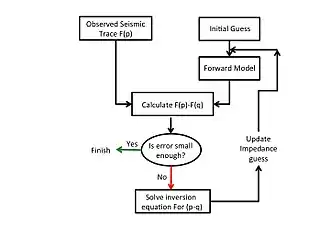
The generalized procedure for inverting any experimental seismic data for ${\displaystyle m=n}$ or ${\displaystyle m>n}$, using the mathematical theory for inverse modeling, as described above, is shown in Fig. 1 and described as follows.

An initial guess of the model impedance is provided to initiate the inversion process. The forward model uses this initial guess to compute a synthetic seismic data which is subtracted from the observed seismic data to calculate the difference vector.

1. An initial guess of the model impedance ${\displaystyle {\vec {q}}}$ is provided to initiate the inversion process.
2. A synthetic seismic data ${\displaystyle {\vec {F}}({\vec {q}})}$ is computed by the forward model, using the model impedance above.
3. The difference vector ${\displaystyle {\vec {F}}({\vec {p}})-{\vec {F}}({\vec {q}})}$ is computed as the difference between experimental and synthetic seismic data.
4. The sensitivity matrix ${\displaystyle \mathbf {A} }$ is computed at this value of the impedance profile.
5. Using ${\displaystyle \mathbf {A} }$ and the difference vector from 3 above, the corrector vector ${\displaystyle \Delta {\vec {p}}}$ is calculated. A new impedance profile is obtained as
   14. ${\displaystyle {\vec {p}}={\vec {q}}+\Delta {\vec {p}}}$
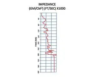
6. The ${\displaystyle L_{1}}$ or ${\displaystyle L_{2}}$ norm of the computed corrector vector is compared with a provided tolerance value. If the computed norm is less than the tolerance, the numerical procedure is concluded and the inverted impedance profile for the earth region is given by ${\displaystyle {\vec {p}}}$ from Eqn. 14. On the other hand, if the norm is greater than the tolerance, iterations through steps 2-6 are repeated but with an updated impedance profile as computed from Eqn. 14. Fig. 2^[7] shows a typical example of impedance profile updating during successive iteration process. According to Cooke and Schneider (1983),^[1] use of the corrected guess from Eqn. 14 as the new initial guess during iteration reduces the error.

Temperature inversion from Marescot (2010)^[8]

We start with an example to invert for earth parameter values from temperature depth distribution in a given earth region. Although this example does not directly relate to seismic inversion since no traveling acoustic waves are involved, it nonetheless introduces practical application of the inversion technique in a manner easy to comprehend, before moving on to seismic applications. In this example, the temperature of the earth is measured at discrete locations in a well bore by placing temperature sensors in the target depths. By assuming a forward model of linear distribution of temperature with depth, two parameters are inverted for from the temperature depth measurements.

The forward model is given by

15. ${\displaystyle {\vec {F}}({\vec {q}})={\vec {T}}=a+bz}$

where ${\displaystyle {\vec {q}}=[a,b]}$. Thus, the dimension of ${\displaystyle {\vec {q}}}$ is 2 i.e. the number of parameters inverted for is 2.

The objective of this inversion algorithm is to find ${\displaystyle {\vec {p}}}$, which is the value of ${\displaystyle [a,b]}$ that minimizes the difference between the observed temperature distribution and those obtained using the forward model of Eqn. 15. Considering the dimension of the forward model or the number of temperature observations to be ${\displaystyle n}$, the components of the forward model is written as

16. ${\displaystyle {\begin{aligned}T_{1}&=a+bz_{1}\\T_{2}&=a+bz_{2}\\\vdots \\T_{n-1}&=a+bz_{n-1}\\T_{n}&=a+bz_{n}\\\end{aligned}}}$
so that ${\displaystyle {\vec {F}}({\vec {q}})=T}$
17. ${\displaystyle \mathbf {A} ={\begin{bmatrix}1&z_{1}\\1&z_{2}\\\vdots &\vdots \\1&z_{n-1}\\1&z_{n}\\\end{bmatrix}}}$

We present results from Marescot (2010)^[8] for the case of ${\displaystyle n=2}$ for which the observed temperature values at depths were ${\displaystyle T_{1}=19^{\circ }C}$ at ${\displaystyle z=2m}$ and ${\displaystyle T_{2}=22^{\circ }C}$ at ${\displaystyle z=8m}$. These experimental data were inverted to obtain earth parameter values of ${\displaystyle a=0.5}$ and ${\displaystyle b=18^{\circ }C}$. For a more general case with large number of temperature observations, Fig. 4 shows the final linear forward model obtained from using the inverted values of ${\displaystyle a}$ and ${\displaystyle b}$. The figure shows a good match between experimental and numerical data.

Wave travel time inversion from Marescot (2010)^[8]

This examples inverts for earth layer velocity from recorded seismic wave travel times. Fig. 5 shows the initial velocity guesses and the travel times recorded from the field, while Fig. 6a shows the inverted heterogeneous velocity model, which is the solution of the inversion algorithm obtained after 30 iterations. As seen in Fig. 6b, there is good comparison between the final travel times obtained from the forward model using the inverted velocity and the field record travel times. Using these solutions, the ray path was reconstructed and is shown to be highly tortuous through the earth model as shown in Fig. 7.

Seismic trace inversion from Cooke and Schneider (1983)

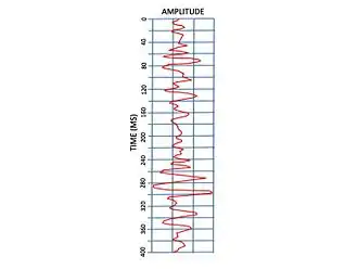
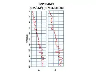
This example, taken from Cooke and Schneider (1983),^[1] shows inversion of a CMP seismic trace for earth model impedance (product of density and velocity) profile. The seismic trace inverted is shown in Fig. 8 while Fig. 9a shows the inverted impedance profile with the input initial impedance used for the inversion algorithm. Also recorded alongside the seismic trace is an impedance log of the earth region as shown in Fig. 9b. The figures show good comparison between the recorded impedance log and the numerical inverted impedance from the seismic trace.

References

- 1 2 3 4 5 6 7 8 9 10 Cooke, D. A.; Schneider W. A. (June 1983). "Generalized linear inversion of reflection seismic data". Geophysics. 48 (6): 665–676. Bibcode:1983Geop...48..665C. doi:10.1190/1.1441497.
- ↑ Pica, A.; Diet J. P.; Tarantola A. (March 1990). "Nonlinear inversion of seismic reflection data in a laterally invariant medium". Geophysics. 55 (3): 284–292. Bibcode:1990Geop...55..284P. doi:10.1190/1.1442836.
- 1 2 3 Francis, A.M. (November 2006). "Understanding Stochastic and Seismic Inversion". First Break. 24 (11). doi:10.3997/1365-2397.2006026.
- 1 2 Wiggins, Ralph (February 1972). "The general linear inverse problem: Implication of surface waves and free oscillations for Earth structure". Reviews of Geophysics. 10 (1): 251–285. Bibcode:1972RvGSP..10..251W. doi:10.1029/RG010i001p00251.
- ↑ Tarantola, A. (1984). "Linearized and inversion of seismic reflection-data". Geophysical Prospecting. 32 (6): 908–1015. doi:10.1111/j.1365-2478.1984.tb00751.x.
- 1 2 3 Kanasewich, E. R.; Chiu S. K. L (June 1985). "Least squares inversion of spatial seismic refraction data". Bulletin of the Seismological Society of America. 75 (3): 865–880.
- ↑ Cooke, D; Cant J. (April 2010). "Model-based seismic inversion: Comparing deterministic and probabilistic approaches". CSEG Recorder.
- 1 2 3 Marescot, Laurent. "Introduction to Inversion in Geophysics". Retrieved 3 May 2013.
Further reading
- Backus, G. 1970. “Inference from inadequate and inaccurate data.” Proceedings of the National Academy of Sciences of the United States of America 65, no. 1.
- Backus, G., and F. Gilbert. 1968. “The Resolving Power of Gross Earth Data.” Geophysical Journal of the Royal Astronomical Society 16 (2): 169–205.
- Backus, G. E., and J. F. Gilbert. 1967. “Numerical applications of a formalism for geophysical inverse problems.” Geophysical Journal of the Royal Astronomical Society. 13 (1-3): 247.
- Bamberger, A., G. Chavent, C. Hemon, and P. Lailly. 1982. “Inversion of normal incidence seisomograms.” Geophysics 47 (5): 757–770.
- Clayton, R. W., and R. H. Stolt. 1981. “A Born-WKBJ inversion method for acoustic reflection data.” Geophysics 46 (11): 1559–1567.
- Franklin, J. N. 1970. “Well-posed stochastic extensions of ill-posed linear problems.” Journal of Mathematical Analysis and Applications 31 (3): 682.
- Parker, R. L. 1977. “Understanding inverse theory.” Annual Review of Earth and planetary sciences 5:35–64.
- Rawlinson, N. 2000. “Inversion of Seismic Dat for Layered Crustal Structure.” Ph.D. diss., Monash University.
- Wang, B., and L. W. Braile. 1996. “Simultaneous inversion of reflection and refraction seismic data and application to field data from the northern Rio Grande rift.” Geophysical Journal International 125 (2): 443–458.
- Weglein, A. B., H. Y. Zhang, A. C. Ramirez, F. Liu, and J. E. M. Lira. 2009. “Clarifying the underlying and fundamental meaning of the approximate linear inversion of seismic data.” Geophysics 74 (6): 6WCD1–WCD13.