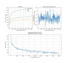
The log-distance path loss model is a radio propagation model that predicts the path loss a signal encounters inside a building or densely populated areas over distance.
Mathematical formulation
Model

Log-distance path loss model is formally expressed as:
where
- is the total path loss in decibels (dB).
- is the transmitted power level, and is the transmitted power.
- is the received power level where is the received power.
- is the path loss in decibels (dB) at the reference distance calculated using the Friis free-space path loss model.
- is the length of the path.
- is the reference distance, usually 1 km (or 1 mile) for a large cell and 1 m to 10 m for a microcell.[1]
- is the path loss exponent.
- is a normal (Gaussian) random variable with zero mean, reflecting the attenuation (in decibels) caused by flat fading. In the case of no fading, this variable is 0. In the case of only shadow fading or slow fading, this random variable may have Gaussian distribution with standard deviation in decibels, resulting in a log-normal distribution of the received power in watts. In the case of only fast fading caused by multipath propagation, the corresponding fluctuation of the signal envelope in volts may be modelled as a random variable with Rayleigh distribution or Ricean distribution[2] (and thus the corresponding power gain may be modelled as a random variable with exponential distribution).
Corresponding non-logarithmic model
This corresponds to the following non-logarithmic gain model:
where is the average multiplicative gain at the reference distance from the transmitter. This gain depends on factors such as carrier frequency, antenna heights and antenna gain, for example due to directional antennas; and is a stochastic process that reflects flat fading. In case of only slow fading (shadowing), it may have log-normal distribution with parameter dB. In case of only fast fading due to multipath propagation, its amplitude may have Rayleigh distribution or Ricean distribution. This can be convenient, because power is proportional to the square of amplitude. Squaring a Rayleigh-distributed random variable produces an exponentially distributed random variable. In many cases, exponential distributions are computationally convenient and allow direct closed-form calculations in many more situations than a Rayleigh (or even a Gaussian).
Empirical coefficient values for indoor propagation
Empirical measurements of coefficients and in dB have shown the following values for a number of indoor wave propagation cases.[3]
| Building type | Frequency of transmission | [dB] | |
|---|---|---|---|
| Vacuum, infinite space | 2.0 | 0 | |
| Retail store | 914 MHz | 2.2 | 8.7 |
| Grocery store | 914 MHz | 1.8 | 5.2 |
| Office with hard partition | 1.5 GHz | 3.0 | 7 |
| Office with soft partition | 900 MHz | 2.4 | 9.6 |
| Office with soft partition | 1.9 GHz | 2.6 | 14.1 |
| Textile or chemical | 1.3 GHz | 2.0 | 3.0 |
| Textile or chemical | 4 GHz | 2.1 | 7.0, 9.7 |
| Office | 60 GHz | 2.2 | 3.92 |
| Commercial | 60 GHz | 1.7 | 7.9 |
See also
References
- ↑ "Log Distance Path Loss or Log Normal Shadowing Model". 30 September 2013.
- ↑ Julius Goldhirsh; Wolfhard J. Vogel. "11.4". Handbook of Propagation Effects for Vehicular and Personal Mobile Satellite Systems (PDF).
- ↑ Wireless communications principles and practices, T. S. Rappaport, 2002, Prentice-Hall