In statistics, modes of variation[1] are a continuously indexed set of vectors or functions that are centered at a mean and are used to depict the variation in a population or sample. Typically, variation patterns in the data can be decomposed in descending order of eigenvalues with the directions represented by the corresponding eigenvectors or eigenfunctions. Modes of variation provide a visualization of this decomposition and an efficient description of variation around the mean. Both in principal component analysis (PCA) and in functional principal component analysis (FPCA), modes of variation play an important role in visualizing and describing the variation in the data contributed by each eigencomponent.[2] In real-world applications, the eigencomponents and associated modes of variation aid to interpret complex data, especially in exploratory data analysis (EDA).
Formulation
Modes of variation are a natural extension of PCA and FPCA.
Modes of variation in PCA
If a random vector has the mean vector , and the covariance matrix with eigenvalues and corresponding orthonormal eigenvectors , by eigendecomposition of a real symmetric matrix, the covariance matrix can be decomposed as
where is an orthogonal matrix whose columns are the eigenvectors of , and is a diagonal matrix whose entries are the eigenvalues of . By the Karhunen–Loève expansion for random vectors, one can express the centered random vector in the eigenbasis
where is the principal component[3] associated with the -th eigenvector , with the properties
- and
Then the -th mode of variation of is the set of vectors, indexed by ,
where is typically selected as .
Modes of variation in FPCA
For a square-integrable random function , where typically and is an interval, denote the mean function by , and the covariance function by
where are the eigenvalues and are the orthonormal eigenfunctions of the linear Hilbert–Schmidt operator
By the Karhunen–Loève theorem, one can express the centered function in the eigenbasis,
where
is the -th principal component with the properties
- and
Then the -th mode of variation of is the set of functions, indexed by ,
that are viewed simultaneously over the range of , usually for .[2]
Estimation
The formulation above is derived from properties of the population. Estimation is needed in real-world applications. The key idea is to estimate mean and covariance.
Modes of variation in PCA
Suppose the data represent independent drawings from some -dimensional population with mean vector and covariance matrix . These data yield the sample mean vector , and the sample covariance matrix with eigenvalue-eigenvector pairs . Then the -th mode of variation of can be estimated by
Modes of variation in FPCA
Consider realizations of a square-integrable random function with the mean function and the covariance function . Functional principal component analysis provides methods for the estimation of and in detail, often involving point wise estimate and interpolation. Substituting estimates for the unknown quantities, the -th mode of variation of can be estimated by
Applications


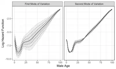
Modes of variation are useful to visualize and describe the variation patterns in the data sorted by the eigenvalues. In real-world applications, modes of variation associated with eigencomponents allow to interpret complex data, such as the evolution of function traits[5] and other infinite-dimensional data.[6] To illustrate how modes of variation work in practice, two examples are shown in the graphs to the right, which display the first two modes of variation. The solid curve represents the sample mean function. The dashed, dot-dashed, and dotted curves correspond to modes of variation with and , respectively.
The first graph displays the first two modes of variation of female mortality data from 41 countries in 2003.[4] The object of interest is log hazard function between ages 0 and 100 years. The first mode of variation suggests that the variation of female mortality is smaller for ages around 0 or 100, and larger for ages around 25. An appropriate and intuitive interpretation is that mortality around 25 is driven by accidental death, while around 0 or 100, mortality is related to congenital disease or natural death.
Compared to female mortality data, modes of variation of male mortality data shows higher mortality after around age 20, possibly related to the fact that life expectancy for women is higher than that for men.
References
- ↑ Castro, P. E.; Lawton, W. H.; Sylvestre, E. A. (November 1986). "Principal Modes of Variation for Processes with Continuous Sample Curves". Technometrics. 28 (4): 329. doi:10.2307/1268982. ISSN 0040-1706. JSTOR 1268982.
- 1 2 Wang, Jane-Ling; Chiou, Jeng-Min; Müller, Hans-Georg (June 2016). "Functional Data Analysis". Annual Review of Statistics and Its Application. 3 (1): 257–295. doi:10.1146/annurev-statistics-041715-033624. ISSN 2326-8298.
- ↑ Kleffe, Jürgen (January 1973). "Principal components of random variables with values in a seperable hilbert space". Mathematische Operationsforschung und Statistik. 4 (5): 391–406. doi:10.1080/02331887308801137. ISSN 0047-6277.
- 1 2 3 "Human Mortality Database". www.mortality.org. Retrieved 2020-03-12.
- ↑ Kirkpatrick, Mark; Heckman, Nancy (August 1989). "A quantitative genetic model for growth, shape, reaction norms, and other infinite-dimensional characters". Journal of Mathematical Biology. 27 (4): 429–450. doi:10.1007/bf00290638. ISSN 0303-6812. PMID 2769086. S2CID 46336613.
- ↑ Jones, M. C.; Rice, John A. (May 1992). "Displaying the Important Features of Large Collections of Similar Curves". The American Statistician. 46 (2): 140–145. doi:10.1080/00031305.1992.10475870. ISSN 0003-1305.