| Part of a series of articles about |
| Calculus |
|---|
Multivariable calculus (also known as multivariate calculus) is the extension of calculus in one variable to calculus with functions of several variables: the differentiation and integration of functions involving multiple variables (multivariate), rather than just one.[1]
Multivariable calculus may be thought of as an elementary part of advanced calculus. For advanced calculus, see calculus on Euclidean space. The special case of calculus in three dimensional space is often called vector calculus.
Introduction
In single-variable calculus, operations like differentiation and integration are made to functions of a single variable. In multivariate calculus, it is required to generalize these to multiple variables, and the domain is therefore multi-dimensional. Care is therefore required in these generalizations, because of two key differences between 1D and higher dimensional spaces:
- There are infinite ways to approach a single point in higher dimensions, as opposed to two (from the positive and negative direction) in 1D;
- There are multiple extended objects associated with the dimension; for example, for a 1D function, it must be represented as a curve on the 2D Cartesian plane, but a function with two variables is a surface in 3D, while curves can also live in 3D space.
The consequence of the first difference is the difference in the definition of the limit and differentiation. Directional limits and derivatives define the limit and differential along a 1D parametrized curve, reducing the problem to the 1D case; further higher-dimensional objects can be constructed from these operators.
The consequence of the second difference is the existence of multiple types of integration, including line integrals, surface integrals and volume integrals. Due to the non-uniqueness of these integrals, an antiderivative or indefinite integral cannot be properly defined.
Limits
A study of limits and continuity in multivariable calculus yields many counterintuitive results not demonstrated by single-variable functions.
A limit along a path may be defined by considering a parametrised path in n-dimensional Euclidean space. Any function can then be projected on the path as a 1D function . The limit of to the point along the path can hence be defined as
-
(1)
Note that the value of this limit can be dependent on the form of , i.e. the path chosen, not just the point which the limit approaches.[1]: 19–22 For example, consider the function . If the point is approached through the line , or in parametric form:
(y))%E2%81%84((x%5E4)%252B(y%5E2)).png.webp)
-
(2)
Then the limit along the path will be:
-
(3)
On the other hand, if the path (or parametrically, ) is chosen, then the limit becomes:
-
(4)
Since taking different paths towards the same point yields different values, a general limit at the point cannot be defined for the function.
A general limit can be defined if the limits to a point along all possible paths converge to the same value, i.e. we say for a function that the limit of to some point is L, if and only if
-
(5)
for all continuous functions such that .
Continuity
From the concept of limit along a path, we can then derive the definition for multivariate continuity in the same manner, that is: we say for a function that is continuous at the point , if and only if
-
(5)
for all continuous functions such that .
As with limits, being continuous along one path does not imply multivariate continuity.
Continuity in each argument not being sufficient for multivariate continuity can also be seen from the following example.[1]: 17–19 For example, for a real-valued function with two real-valued parameters, , continuity of in for fixed and continuity of in for fixed does not imply continuity of .
Consider
It is easy to verify that this function is zero by definition on the boundary and outside of the quadrangle . Furthermore, the functions defined for constant and and by
- and
are continuous. Specifically,
- for all x and y. Therefore, and moreover, along the coordinate axes, and . Therefore the function is continuous along both individual arguments.
However, consider the parametric path . The parametric function becomes
-
(6)
Therefore,
-
(7)
It is hence clear that the function is not multivariate continuous, despite being continuous in both coordinates.
Theorems regarding multivariate limits and continuity
- All properties of linearity and superposition from single-variable calculus carry over to multivariate calculus.
- Composition: If and are both multivariate continuous functions at the points and respectively, then is also a multivariate continuous function at the point .
- Multiplication: If and are both continuous functions at the point , then is continuous at , and is also continuous at provided that .
- If is a continuous function at point , then is also continuous at the same point.
- If is Lipschitz continuous (with the appropiate normed spaces as needed) in the neighbourhood of the point , then is multivariate continuous at .
Proof | |||||||
|---|---|---|---|---|---|---|---|
|
From the Lipschitz continuity condition for we have
where is the Lipschitz constant. Note also that, as is continuous at , for every there exists a such that . Hence, for every , choose ; there exists an such that for all satisfying , , and . Hence converges to regardless of the precise form of . |
Differentiation
Directional derivative
The derivative of a single-variable function is defined as
-
(9)
Using the extension of limits discussed above, one can then extend the definition of the derivative to a scalar-valued function along some path :
-
(10)
Unlike limits, for which the value depends on the exact form of the path , it can be shown that the derivative along the path depends only on the tangent vector of the path at , i.e. , provided that is Lipschitz continuous at , and that the limit exits for at least one such path.
Proof | |||||||||||||||||||||
|---|---|---|---|---|---|---|---|---|---|---|---|---|---|---|---|---|---|---|---|---|---|
|
For continuous up to the first derivative (this statement is well defined as is a function of one variable), we can write the Taylor expansion of around using Taylor's theorem to construct the remainder:
where . Substituting this into 10,
where . Lipschitz continuity gives us for some finite , . It follows that . Note also that given the continuity of , as . Substituting these two conditions into 12,
whose limit depends only on as the dominant term. |
It is therefore possible to generate the definition of the directional derivative as follows: The directional derivative of a scalar-valued function along the unit vector at some point is
-
(14)
or, when expressed in terms of ordinary differentiation,
-
(15)
which is a well defined expression because is a scalar function with one variable in .
It is not possible to define a unique scalar derivative without a direction; it is clear for example that . It is also possible for directional derivatives to exist for some directions but not for others.
Partial derivative
The partial derivative generalizes the notion of the derivative to higher dimensions. A partial derivative of a multivariable function is a derivative with respect to one variable with all other variables held constant.[1]: 26ff
A partial derivative may be thought of as the directional derivative of the function along a coordinate axis.
Partial derivatives may be combined in interesting ways to create more complicated expressions of the derivative. In vector calculus, the del operator () is used to define the concepts of gradient, divergence, and curl in terms of partial derivatives. A matrix of partial derivatives, the Jacobian matrix, may be used to represent the derivative of a function between two spaces of arbitrary dimension. The derivative can thus be understood as a linear transformation which directly varies from point to point in the domain of the function.
Differential equations containing partial derivatives are called partial differential equations or PDEs. These equations are generally more difficult to solve than ordinary differential equations, which contain derivatives with respect to only one variable.[1]: 654ff
Multiple integration
The multiple integral expands the concept of the integral to functions of any number of variables. Double and triple integrals may be used to calculate areas and volumes of regions in the plane and in space. Fubini's theorem guarantees that a multiple integral may be evaluated as a repeated integral or iterated integral as long as the integrand is continuous throughout the domain of integration.[1]: 367ff
The surface integral and the line integral are used to integrate over curved manifolds such as surfaces and curves.
Fundamental theorem of calculus in multiple dimensions
In single-variable calculus, the fundamental theorem of calculus establishes a link between the derivative and the integral. The link between the derivative and the integral in multivariable calculus is embodied by the integral theorems of vector calculus:[1]: 543ff
In a more advanced study of multivariable calculus, it is seen that these four theorems are specific incarnations of a more general theorem, the generalized Stokes' theorem, which applies to the integration of differential forms over manifolds.[2]
Applications and uses
Techniques of multivariable calculus are used to study many objects of interest in the material world. In particular,
| Type of functions | Applicable techniques | ||
|---|---|---|---|
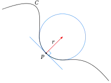
| Curves |  | for | Lengths of curves, line integrals, and curvature. |
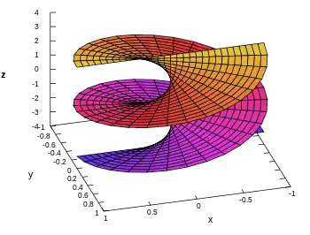
| Surfaces |  | for | Areas of surfaces, surface integrals, flux through surfaces, and curvature. |
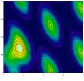
| Scalar fields |  | Maxima and minima, Lagrange multipliers, directional derivatives, level sets. | |
| Vector fields |  | Any of the operations of vector calculus including gradient, divergence, and curl. |
Multivariable calculus can be applied to analyze deterministic systems that have multiple degrees of freedom. Functions with independent variables corresponding to each of the degrees of freedom are often used to model these systems, and multivariable calculus provides tools for characterizing the system dynamics.
Multivariate calculus is used in the optimal control of continuous time dynamic systems. It is used in regression analysis to derive formulas for estimating relationships among various sets of empirical data.
Multivariable calculus is used in many fields of natural and social science and engineering to model and study high-dimensional systems that exhibit deterministic behavior. In economics, for example, consumer choice over a variety of goods, and producer choice over various inputs to use and outputs to produce, are modeled with multivariate calculus.
Non-deterministic, or stochastic systems can be studied using a different kind of mathematics, such as stochastic calculus.
See also
References
External links
- UC Berkeley video lectures on Multivariable Calculus, Fall 2009, Professor Edward Frenkel
- MIT video lectures on Multivariable Calculus, Fall 2007
- Multivariable Calculus: A free online textbook by George Cain and James Herod
- Multivariable Calculus Online: A free online textbook by Jeff Knisley
- Multivariable Calculus – A Very Quick Review, Prof. Blair Perot, University of Massachusetts Amherst
- Multivariable Calculus, Online text by Dr. Jerry Shurman