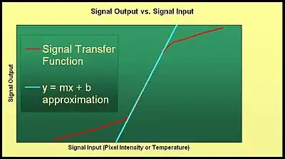
The signal transfer function (SiTF) is a measure of the signal output versus the signal input of a system such as an infrared system or sensor. There are many general applications of the SiTF. Specifically, in the field of image analysis, it gives a measure of the noise of an imaging system, and thus yields one assessment of its performance.^[1]

SiTF evaluation

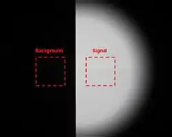
In evaluating the SiTF curve, the signal input and signal output are measured differentially; meaning, the differential of the input signal and differential of the output signal are calculated and plotted against each other. An operator, using computer software, defines an arbitrary area, with a given set of data points, within the signal and background regions of the output image of the infrared sensor, i.e. of the unit under test (UUT), (see "Half Moon" image below). The average signal and background are calculated by averaging the data of each arbitrarily defined region. A second order polynomial curve is fitted to the data of each line. Then, the polynomial is subtracted from the average signal and background data to yield the new signal and background. The difference of the new signal and background data is taken to yield the net signal. Finally, the net signal is plotted versus the signal input. The signal input of the UUT is within its own spectral response. (e.g. color-correlated temperature, pixel intensity, etc.). The slope of the linear portion of this curve is then found using the method of least squares.^[2]

SiTF curve

The red line is the SiTF. As can be seen, a line is fitted to the linear portion of the signal output versus signal input of an infrared sensor.

Half moon target – on the left the image of the background region and on the right an image of the signal region. Using specialized software, an operator arbitrarily defines an area of evaluation in both regions to be used in determining the signal transfer function.

The net signal is calculated from the average signal and background, as in signal to noise ratio (imaging)#Calculations. The SiTF curve is then given by the signal output data, (net signal data), plotted against the signal input data (see graph of SiTF to the right). All the data points in the linear region of the SiTF curve can be used in the method of least squares to find a linear approximation. Given ${\displaystyle n\,}$ data points ${\displaystyle (x_{i}\,,y_{i}\,)}$ a best fit line parameterized as ${\displaystyle y=mx+b\,}$ is given by:^[3]

${\displaystyle m={\frac {{\frac {\sum x_{i}y_{i}}{n}}-{\frac {\sum x_{i}}{n}}{\frac {\sum y_{i}}{n}}}{{\frac {\sum x_{i}^{2}}{n}}-({\frac {\sum x_{i}}{n}})^{2}}}\qquad \qquad b={\frac {\sum y_{i}}{n}}-m{\frac {\sum x_{i}}{n}}}$

See also

• Optical transfer function
• Distortion
• Minimum resolvable temperature difference
• Noise equivalent temperature difference
• Power spectral density
• Minimum resolvable contrast
• Signal to noise ratio (imaging)

References

External links

• http://www.electro-optical.com

References

- ↑ Tom L. Williams (1998). The Optical Transfer Function of Imaging Systems. CRC Press. ISBN 0-7503-0599-1.
- ↑ Electro Optical Industries, Inc.(2005). EO TestLab Methodology. In Education.
- ↑ Aboufadel, E. F., Goldberg, J. L., Potter, M. C. (2005).Advanced Engineering Mathematics (3rd ed.).New York, New York: Oxford University Press