EMG

Probability density function
Cumulative distribution function
Parameters	μ ∈ R — mean of Gaussian component σ2 > 0 — variance of Gaussian component λ > 0 — rate of exponential component
Support	x ∈ R
PDF	${\displaystyle {\frac {\lambda }{2}}e^{{\frac {\lambda }{2}}(2\mu +\lambda \sigma ^{2}-2x)}\operatorname {erfc} \left({\frac {\mu +\lambda \sigma ^{2}-x}{{\sqrt {2}}\sigma }}\right)}$
CDF	${\displaystyle \Phi (x,\mu ,\sigma )-{\frac {1}{2}}e^{{\frac {\lambda }{2}}(2\mu +\lambda \sigma ^{2}-2x)}\operatorname {erfc} \left({\frac {\mu +\lambda \sigma ^{2}-x}{{\sqrt {2}}\sigma }}\right)}$ where ${\displaystyle \Phi (x,\mu ,\sigma )}$ is the CDF of a Gaussian distribution
Mean	${\displaystyle \mu +1/\lambda }$
Mode	${\displaystyle x_{m}=\mu -\operatorname {sgn} \left(\tau \right){\sqrt {2}}\sigma \operatorname {erfcxinv} \left({\frac {{|}\tau {|}}{\sigma }}{\sqrt {\frac {2}{\pi }}}\right)+{\frac {\sigma ^{2}}{\tau }}}$ ${\displaystyle f(x_{m})=h\exp \left(-{\frac {1}{2}}\left({\frac {\mu -x_{m}}{\sigma }}\right)^{2}\right)}$
Variance	${\displaystyle \sigma ^{2}+1/\lambda ^{2}}$
Skewness	${\displaystyle {\frac {2}{\sigma ^{3}\lambda ^{3}}}\left(1+{\frac {1}{\sigma ^{2}\lambda ^{2}}}\right)^{-3/2}}$
Ex. kurtosis	${\displaystyle {\frac {3(1+{\frac {2}{\sigma ^{2}\lambda ^{2}}}+{\frac {3}{\lambda ^{4}\sigma ^{4}}})}{\left(1+{\frac {1}{\lambda ^{2}\sigma ^{2}}}\right)^{2}}}-3}$
MGF	${\displaystyle \left(1-{\frac {t}{\lambda }}\right)^{-1}\,\exp \left(\mu t+{\frac {1}{2}}\sigma ^{2}t^{2}\right)}$
CF	${\displaystyle \left(1-{\frac {it}{\lambda }}\right)^{-1}\,\exp \left(i\mu t-{\frac {1}{2}}\sigma ^{2}t^{2}\right)}$

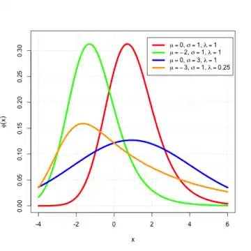
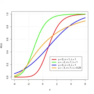
In probability theory, an exponentially modified Gaussian distribution (EMG, also known as exGaussian distribution) describes the sum of independent normal and exponential random variables. An exGaussian random variable Z may be expressed as Z = X + Y, where X and Y are independent, X is Gaussian with mean μ and variance σ², and Y is exponential of rate λ. It has a characteristic positive skew from the exponential component.

It may also be regarded as a weighted function of a shifted exponential with the weight being a function of the normal distribution.

Definition

The probability density function (pdf) of the exponentially modified normal distribution is^[1]

${\displaystyle f(x;\mu ,\sigma ,\lambda )={\frac {\lambda }{2}}e^{{\frac {\lambda }{2}}(2\mu +\lambda \sigma ^{2}-2x)}\operatorname {erfc} \left({\frac {\mu +\lambda \sigma ^{2}-x}{{\sqrt {2}}\sigma }}\right),}$

where erfc is the complementary error function defined as

${\displaystyle {\begin{aligned}\operatorname {erfc} (x)&=1-\operatorname {erf} (x)\\&={\frac {2}{\sqrt {\pi }}}\int _{x}^{\infty }e^{-t^{2}}\,dt.\end{aligned}}}$

This density function is derived via convolution of the normal and exponential probability density functions.

Alternative forms for computation

An alternative but equivalent form of the EMG distribution is used for description of peak shape in chromatography.^[2] This is as follows

${\displaystyle f(x;h,\mu ,\sigma ,\tau )={\frac {h\sigma }{\tau }}{\sqrt {\frac {\pi }{2}}}\exp \left({\frac {1}{2}}\left({\frac {\sigma }{\tau }}\right)^{2}-{\frac {x-\mu }{\tau }}\right)\operatorname {erfc} \left({\frac {1}{\sqrt {2}}}\ \left({\frac {\sigma }{\tau }}-{\frac {x-\mu }{\sigma }}\right)\right),}$

(1)

where

${\displaystyle h}$ is the amplitude of Gaussian,

${\displaystyle \tau ={\frac {1}{\lambda }}}$ is exponent relaxation time, ${\displaystyle \tau ^{2}}$ is a variance of exponential probability density function.

This function cannot be calculated for some values of parameters (for example, ${\displaystyle \tau =0}$) because of arithmetic overflow. Alternative, but equivalent form of writing the function was proposed by Delley:^[3]

${\displaystyle f(x;h,\mu ,\sigma ,\tau )=h\exp \left(-{\frac {1}{2}}\left({\frac {x-\mu }{\sigma }}\right)^{2}\right){\frac {\sigma }{\tau }}{\sqrt {\frac {\pi }{2}}}\operatorname {erfcx} \left({\frac {1}{\sqrt {2}}}\ \left({\frac {\sigma }{\tau }}-{\frac {x-\mu }{\sigma }}\right)\right),}$

(2)

where ${\displaystyle \operatorname {erfcx} t=\exp t^{2}\cdot \operatorname {erfc} t}$ is a scaled complementary error function

In the case of this formula arithmetic overflow is also possible, region of overflow is different from the first formula, except for very small τ.

For small τ it is reasonable to use asymptotic form of the second formula:

${\displaystyle f(x;h,\mu ,\sigma ,\tau )={\frac {h\exp \left(-{\frac {1}{2}}\left({\frac {x-\mu }{\sigma }}\right)^{2}\right)}{1+{\frac {\left(x-\mu \right)\tau }{\sigma ^{2}}}}},}$

(3)

Decision on formula usage is made on the basis of the parameter ${\displaystyle z={\frac {1}{\sqrt {2}}}\left({\frac {\sigma }{\tau }}-{\frac {x-\mu }{\sigma }}\right)}$:

for z < 0 computation should be made^[2] according to the first formula,

for 0 ≤ z ≤ 6.71·10⁷ (in the case of double-precision floating-point format) according to the second formula,

and for z > 6.71·10⁷ according to the third formula.

Mode (position of apex, most probable value) is calculated^[2] using derivative of formula 2; the inverse of scaled complementary error function erfcxinv() is used for calculation. Approximate values are also proposed by Kalambet et al.^[2] Though the mode is at a value higher than that of the original Gaussian, the apex is always located on the original (unmodified) Gaussian.

Parameter estimation

There are three parameters: the mean of the normal distribution (μ), the standard deviation of the normal distribution (σ) and the exponential decay parameter (τ = 1 / λ). The shape K = τ / σ is also sometimes used to characterise the distribution. Depending on the values of the parameters, the distribution may vary in shape from almost normal to almost exponential.

The parameters of the distribution can be estimated from the sample data with the method of moments as follows:^[4][5]

${\displaystyle m=\mu +\tau ,}$

${\displaystyle s^{2}=\sigma ^{2}+\tau ^{2},}$

${\displaystyle \gamma _{1}={\frac {2\tau ^{3}}{(\sigma ^{2}+\tau ^{2})^{3/2}}},}$

where m is the sample mean, s is the sample standard deviation, and γ₁ is the skewness.

Solving these for the parameters gives:

${\displaystyle {\hat {\mu }}=m-s\left({\frac {\gamma _{1}}{2}}\right)^{1/3},}$

${\displaystyle {\hat {\sigma ^{2}}}=s^{2}\left[1-\left({\frac {\gamma _{1}}{2}}\right)^{2/3}\right],}$

${\displaystyle {\hat {\tau }}=s\left({\frac {\gamma _{1}}{2}}\right)^{1/3}.}$

Occurrence

The distribution is used as a theoretical model for the shape of chromatographic peaks.^[1][2][12] It has been proposed as a statistical model of intermitotic time in dividing cells.^[13][14] It is also used in modelling cluster ion beams.^[15] It is commonly used in psychology and other brain sciences in the study of response times.^[16][17][18] In a slight variant where the mean of the Normal component is set to zero, it is also used in Stochastic Frontier Analysis, as one of the distributional specifications for the composed error term that models inefficiency.^[19] In signal processing, EMGs have been extended to the multimodal case with an optional oscillation term to represent digitized sound signals.^[8]

Related distributions

This family of distributions is a special or limiting case of the normal-exponential-gamma distribution. This can also be seen as a three-parameter generalization of a normal distribution to add skew; another distribution like that is the skew normal distribution, which has thinner tails. The distribution is a compound probability distribution in which the mean of a normal distribution varies randomly as a shifted exponential distribution.

A Gaussian minus exponential distribution has been suggested for modelling option prices.^[20] If such a random variable Y has parameters μ, σ, λ, then its negative -Y has an exponentially modified Gaussian distribution with parameters -μ, σ, λ, and thus Y has mean ${\displaystyle \mu -{\tfrac {1}{\lambda }}}$ and variance ${\displaystyle \sigma ^{2}+{\tfrac {1}{\lambda ^{2}}}}$.

References

- 1 2 Grushka, Eli (1972). "Characterization of Exponentially Modified Gaussian Peaks in Chromatography". Analytical Chemistry. 44 (11): 1733–1738. doi:10.1021/ac60319a011. PMID 22324584.
- 1 2 3 4 5 Kalambet, Y.; Kozmin, Y.; Mikhailova, K.; Nagaev, I.; Tikhonov, P. (2011). "Reconstruction of chromatographic peaks using the exponentially modified Gaussian function". Journal of Chemometrics. 25 (7): 352. doi:10.1002/cem.1343. S2CID 121781856.
- ↑ Delley, R (1985). "Series for the Exponentially Modified Gaussian Peak Shape". Anal. Chem. 57: 388. doi:10.1021/ac00279a094.
- ↑ Dyson, N. A. (1998). Chromatographic Integration Methods. Royal Society of Chemistry, Information Services. p. 27. ISBN 9780854045105. Retrieved 2015-05-15.
- ↑ Olivier J. and Norberg M. M. (2010) Positively skewed data: Revisiting the Box−Cox power transformation. Int. J. Psych. Res. 3 (1) 68−75.
- ↑ Ratcliff, R (1979). "Group reaction time distributions and an analysis of distribution statistics". Psychol. Bull. 86 (3): 446–461. CiteSeerX 10.1.1.409.9863. doi:10.1037/0033-2909.86.3.446. PMID 451109.
- ↑ Vincent, S. B. (1912). "The functions of the vibrissae in the behaviour of the white rat". Animal Behaviour Monographs. 1 (5): 7–81.
- 1 2 Hahne, C. (2022). "Multimodal Exponentially Modified Gaussian Oscillators". IEEE International Ultrasonic Symposium 2022 (IUS): 1–4. arXiv:2209.12202.
- ↑ "MEMG on GitHub". GitHub.
- ↑ Heathcote, A (1996). "RTSYS: A DOS application for the analysis of reaction time data". Behavior Research Methods, Instruments, & Computers. 28 (3): 427–445. doi:10.3758/bf03200523. hdl:1959.13/28044.
- ↑ Ulrich, R.; Miller, J. (1994). "Effects of outlier exclusion on reaction time analysis". J. Exp. Psych.: General. 123 (1): 34–80. doi:10.1037/0096-3445.123.1.34. PMID 8138779.
- ↑ Gladney, HM; Dowden, BF; Swalen, JD (1969). "Computer-Assisted Gas-Liquid Chromatography". Anal. Chem. 41 (7): 883–888. doi:10.1021/ac60276a013.
- ↑ Golubev, A. (2010). "Exponentially modified Gaussian (EMG) relevance to distributions related to cell proliferation and differentiation". Journal of Theoretical Biology. 262 (2): 257–266. Bibcode:2010JThBi.262..257G. doi:10.1016/j.jtbi.2009.10.005. PMID 19825376.
- ↑ Tyson, D. R.; Garbett, S. P.; Frick, P. L.; Quaranta, V. (2012). "Fractional proliferation: A method to deconvolve cell population dynamics from single-cell data". Nature Methods. 9 (9): 923–928. doi:10.1038/nmeth.2138. PMC 3459330. PMID 22886092.
- ↑ Nicolaescu, D.; Takaoka, G. H.; Ishikawa, J. (2006). "Multiparameter characterization of cluster ion beams". Journal of Vacuum Science & Technology B: Microelectronics and Nanometer Structures. 24 (5): 2236. Bibcode:2006JVSTB..24.2236N. doi:10.1116/1.2335433.
- ↑ Palmer, EM; Horowitz Todd, S; Torralba, A; Wolfe, JM (2011). "What are the shapes of response time distributions in visual search?". J Exp Psychol. 37 (1): 58–71. doi:10.1037/a0020747. PMC 3062635. PMID 21090905.
- ↑ Rohrer, D; Wixted, JT (1994). "An analysis of latency and interresponse time in free recall". Memory & Cognition. 22 (5): 511–524. doi:10.3758/BF03198390. PMID 7968547.
- ↑ Soltanifar, M; Escobar, M; Dupuis, A; Schachar, R (2021). "A Bayesian Mixture Modelling of Stop Signal Reaction Time Distributions: The Second Contextual Solution for the Problem of Aftereffects of Inhibition on SSRT Estimations". Brain Sciences. 11 (9): 1–26. doi:10.3390/brainsci11081102. PMC 8391500. PMID 34439721.
- ↑ Lovell, Knox CA; S.C. Kumbhakar (2000). Stochastic Frontier Analysis. Cambridge University Press. pp. 80–82. ISBN 0-521-48184-8.
- ↑ Peter Carr and Dilip B. Madan, Saddlepoint Methods for Option Pricing, The Journal of Computational Finance (49–61) Volume 13/Number 1, Fall 2009