| Part of a series on |
| Artificial intelligence |
|---|
 |
Applications of machine learning in earth sciences include geological mapping, gas leakage detection and geological features identification. Machine learning (ML) is a type of artificial intelligence (AI) that enables computer systems to classify, cluster, identify and analyze vast and complex sets of data while eliminating the need for explicit instructions and programming.[1] Earth science is the study of the origin, evolution, and future[2] of the planet Earth. The Earth system can be subdivided into four major components including the solid earth, atmosphere, hydrosphere and biosphere.[3]
A variety of algorithms may be applied depending on the nature of the earth science exploration. Some algorithms may perform significantly better than others for particular objectives. For example, convolutional neural networks (CNN) are good at interpreting images, artificial neural networks (ANN) perform well in soil classification[4] but more computationally expensive to train than support-vector machine (SVM) learning. The application of machine learning has been popular in recent decades, as the development of other technologies such as unmanned aerial vehicles (UAVs),[5] ultra-high resolution remote sensing technology and high-performance computing units[6] lead to the availability of large high-quality datasets and more advanced algorithms.
Significance
Complexity of earth science
Problems in earth science are often complex.[7] It is difficult to apply well-known and described mathematical models to the natural environment, therefore machine learning is commonly a better alternative for such non-linear problems.[8] Ecological data are commonly non-linear and consist of higher-order interactions, and together with missing data, traditional statistics may underperform as unrealistic assumptions such as linearity are applied to the model.[9][10] A number of researchers found that machine learning outperforms traditional statistical models in earth science, such as in characterizing forest canopy structure,[11] predicting climate-induced range shifts,[12] and delineating geologic facies.[13] Characterizing forest canopy structure enables scientists to study vegetation response to climate change.[14] Predicting climate-induced range shifts enable policy makers to adopt suitable conversation method to overcome the consequences of climate change.[15] Delineating geologic facies helps geologists to understand the geology of an area, which is essential for the development and management of an area.[16]
Inaccessible data
In Earth Sciences, some data are often difficult to access or collect, therefore inferring data from data that are easily available by machine learning method is desirable.[10] For example, geological mapping in tropical rainforests is challenging because the thick vegetation cover and rock outcrops are poorly exposed.[17] Applying remote sensing with machine learning approaches provides an alternative way for rapid mapping without the need of manually mapping in the unreachable areas.[17]
Reduce time costs
Machine learning can also reduce the efforts done by experts, as manual tasks of classification and annotation etc are the bottlenecks in the workflow of the research of earth science.[10] Geological mapping, especially in a vast, remote area is labour, cost and time-intensive with traditional methods.[18] Incorporation of remote sensing and machine learning approaches can provide an alternative solution to eliminate some field mapping needs.[18]
Consistent and bias-free
Consistency and bias-free is also an advantage of machine learning compared to manual works by humans. In research comparing the performance of human and machine learning in the identification of dinoflagellates, machine learning is found to be not as prone to systematic bias as humans.[19] A recency effect that is present in humans is that the classification often biases towards the most recently recalled classes.[19] In a labelling task of the research, if one kind of dinoflagellates occurs rarely in the samples, then expert ecologists commonly will not classify it correctly.[19] The systematic bias strongly deteriorate the classification accuracies of humans.[19]
Optimal machine learning algorithm
The extensive usage of machine learning in various fields has led to a wide range of algorithms of learning methods being applied. The machine learning algorithm applied in solving earth science problem in much interest to the researchers.[20][4][7] Choosing the optimal algorithm for a specific purpose can lead to a significant boost in accuracy.[21] For example, the lithological mapping of gold-bearing granite-greenstone rocks in Hutti, India with AVIRIS-NG hyperspectral data, shows more than 10% difference in overall accuracy between using Support Vector Machine (SVM) and random forest.[22] Some algorithms can also reveal some important information. 'White-box models' are transparent models in which the results and methodologies can be easily explained, while 'black-box' models are the opposite.[21] For example, although the support-vector machine (SVM) yielded the best result in landslide susceptibility assessment accuracy, the result cannot be rewritten in the form of expert rules that explain how and why an area was classified as that specific class.[7] In contrast, the decision tree has a transparent model that can be understood easily, and the user can observe and fix the bias if any present in the model.[7] If the computational power is a concern, a more computationally demanding learning method such as artificial neural network is less preferred despite the fact that artificial neural network may slightly outperform other algorithms, such as in soil classification.[4]
Below are highlights of some commonly applied algorithms.[23]
 Support Vector Machine (SVM)
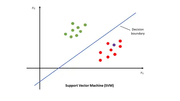
In the Support Vector Machine (SVM), the decision boundary was determined during the training process by the training dataset as represented by the green and red dots. The data of purple falls below the decision boundary, therefore it belongs to the red class.[7]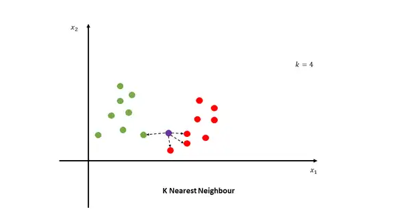 K nearest neighbor
K nearest neighbor classifies data based on their similarities. k is a parameter representing the number of neighbors that will be considered for the voting process. For example, in the figure k = 4, therefore the nearest 4 neighbors are considered. In the 4 nearest neighbors, 3 belong to the red class and 1 belongs to the green class. The purple data is classified as the red class.[24]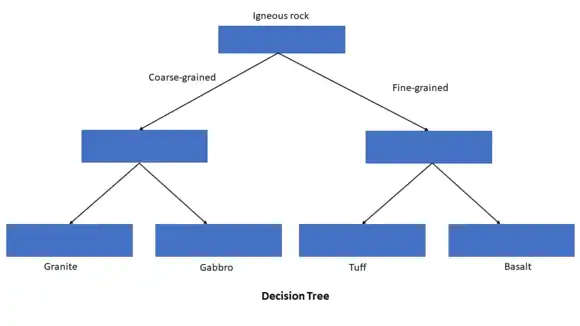 Decision Tree
Decision Tree shows the possible outcomes of related choices. Decision Tree can further be divided into Classification Tree and Regression Tree. The above figure shows a Classification Tree as the outputs are discrete classes. For regression Tree, the output is a number. This is a white-box model which is transparent and the user is able to spot out the bias if any appears in the model.[7]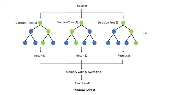 Random forest
In random forest, multiple decision trees are used together in an ensemble method. Multiple decision trees are produced during the training of a model. Different decision trees may give up various results. The majority voting/ averaging process gives out the final result. This method yields a higher accuracy of using a single decision tree only.[22]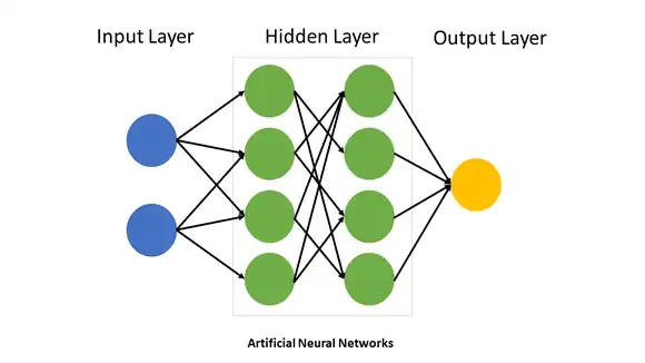 Neural Networks
Neural Networks mimic neurons in a biological brain. It consists of multiple layers, where the layers in between are hidden layers. The weights of the connections are adjusted during the training process. As the logic in between is unclear, it is referred to as 'black-box operation'. Convolutional neural network (CNN) is a subclass of Neural Networks, which is commonly used for processing images.[24]
Usage
Mapping
Geological or lithological mapping and mineral prospectivity mapping
Geological or lithological mapping produces maps showing geological features and geological units. Mineral prospectivity mapping utilizes a variety of datasets such as geological maps, aeromagnetic imagery, etc to produce maps that are specialized for mineral exploration. Geological/ Lithological Mapping and Mineral Prospectivity Mapping can be carried out by processing the data with machine-learning techniques with the input of spectral imagery obtained from remote sensing and geophysical data.[25] Spectral imagery is the imaging of selected electromagnetic wavelength bands in the electromagnetic spectrum, while conventional imaging captures three wavelength bands (Red, Green, Blue) in the electromagnetic spectrum.[26] Random Forest and Support Vector Machine (SVM) etc are common algorithms being used with remote sensed geophysical data, while Simple Linear Iterative Clustering-Convolutional Neural Network (SLIC-CNN)[5] and Convolutional Neural Networks (CNN)[18] etc are commonly applied while dealing with aerial photos and images. Large scale mapping can be carried out with geophysical data from airborne and satellite remote sensing geophysical data,[22] and smaller-scale mapping can be carried out with images from Unmanned Aerial Vehicle (UAV) for higher resolution.[5]
Vegetation cover is one of the major obstacles for geological mapping with remote sensing, as reported in various research, both in large-scale and small-scale mapping. Vegetation affects the quality of spectral image[25] or obscures the rock information in the aerial images.[5]
| Objective | Input dataset | Location | Machine Learning Algorithms (MLAs) | Performance |
|---|---|---|---|---|
| Lithological Mapping of Gold-bearing granite-greenstone rocks[22] | AVIRIS-NG hyperspectral data | Hutti, India | Linear Discriminant Analysis (LDA), | Support Vector Machine (SVM) outperforms the other Machine Learning Algorithms (MLAs) |
| Lithological Mapping in the Tropical Rainforest[17] | Magnetic Vector Inversion,
Ternary RGB map, Shuttle Radar Topography Mission (SRTM), False color (RGB) of Landsat 8 combining bands 4, 3 and 2 |
Cinzento Lineament, Brazil | Random Forest | Two predictive maps were generated:
(1) Map generated with remote sensing data only has a 52.7% accuracy when compared to the geological map, but several new possible lithological units are identified (2) Map generated with remote sensing data and spatial constraints has a 78.7% accuracy but no new possible lithological units are identified |
| Geological Mapping for mineral exploration[27] | Airborne polarimetric Terrain Observation with Progressive Scans SAR (TopSAR),
geophysical data |
Western Tasmania | Random Forest | Low reliability of TopSAR for geological mapping, but accurate with geophysical data. |
| Geological and Mineralogical mapping | Multispectral and hyperspectral satellite data | Central Jebilet,
Morocco |
Support Vector Machine (SVM) | The accuracy of using hyperspectral data for classifying is slightly higher than that using multispectral data, obtaining 93.05% and 89.24% respectively, showing that machine learning is a reliable tool for mineral exploration. |
| Integrating Multigeophysical Data into a Cluster Map[28] | Airborne magnetic,
frequency electromagnetic, radiometric measurements, ground gravity measurements |
Trøndelag, Mid-Norway | Random Forest | The cluster map produced has a satisfactory relationship with the existing geological map but with minor misfits. |
| High-Resolution Geological Mapping with Unmanned Aerial Vehicle (UAV)[5] | Ultra-resolution RGB images | Taili waterfront,
Liaoning Province, China |
Simple Linear Iterative Clustering-Convolutional Neural Network (SLIC-CNN) | The result is satisfactory in mapping major geological units but showed poor performance in mapping pegmatites, fine-grained rocks and dykes. UAVs were unable to collect rock information where the rocks were not exposed. |
| Surficial Geology Mapping[18]
Remote Predictive Mapping (RPM) |
Aerial Photos,
Landsat Reflectance, High-Resolution Digital Elevation Data |
South Rae Geological Region,
Northwest Territories, Canada |
Convolutional Neural Networks (CNN),
Random Forest |
The resulting accuracy of CNN was 76% in the locally trained area, while 68% for an independent test area. The CNN achieved a slightly higher accuracy of 4% than the Random Forest. |
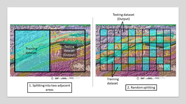
As the training of machine learning for landslide susceptibility mapping requires both training and testing dataset, therefore splitting of the dataset is required. Two splitting methods for the datasets are presented on the geologic map of the east Cumberland Gap. The method presented on the left, 'Splitting into two adjacent areas' is more useful as the automation algorithm can carry out mapping of a new area with the input of expert processed data of adjacent land. The cyan coloured pixels show the training dataset while the remaining shows the testing datasets.
Landslide susceptibility and hazard mapping
Landslide susceptibility refers to the probability of landslide of a place, which is affected by the local terrain conditions.[29] Landslide susceptibility mapping can highlight areas prone to landslide risks which are useful for urban planning and disaster management works.[7] Input dataset for machine learning algorithms usually includes topographic information, lithological information, satellite images, etc. and some may include land use, land cover, drainage information, vegetation cover[7][30][31][32] according to their study needs. In machine learning training for landslide susceptibility mapping, training and testing datasets are required.[7] There are two methods of allocating datasets for training and testing, one is to random split the study area for the datasets, another is to split the whole study into two adjacent parts for the two datasets. To test the classification models, the common practice is to split the study area randomly into two datasets,[7][33] however, it is more useful that the study area can be split into two adjacent parts so that the automation algorithm can carry out mapping of a new area with the input of expert processed data of adjacent land.[7]
| Objective | Input dataset | Location | Machine Learning Algorithms (MLAs) | Performance |
|---|---|---|---|---|
| Landslide Susceptibility Assessment[7] | Digital Elevation Model (DEM),
Geological Map, 30m Landsat Imagery |
Fruška Gora Mountain,
Serbia |
Support Vector Machine (SVM), | Support Vector Machine (SVM) outperforms the others |
| Landslide Susceptibility Mapping[33] | ASTER satellite-based geomorphic data,
geological maps |
Honshu Island,
Japan |
Artificial Neural Network (ANN) | Accuracy greater than 90% for determining the probability of landslide. |
| Landslide Susceptibility Zonation through ratings[30] | Spatial data layers with
slope, aspect, relative relief, lithology, structural features, land use, land cover, drainage density |
Parts of Chamoli and Rudraprayag districts of the State of Uttarakhand,
India |
Artificial Neural Network (ANN) | The AUC of this approach reaches 0.88. This approach generated an accurate assessment of landslide risks. |
| Regional Landslide Hazard Analysis[31] | Topographic slope,
topographic aspect, topographic curvature, distance from drainage, lithology, distance from lineament, land cover from TM satellite images, Vegetation index (NDVI), precipitation data |
The eastern part of Selangor state,
Malaysia |
Artificial Neural Network (ANN) | The approach achieved 82.92% accuracy of prediction. |
Feature identification and detection
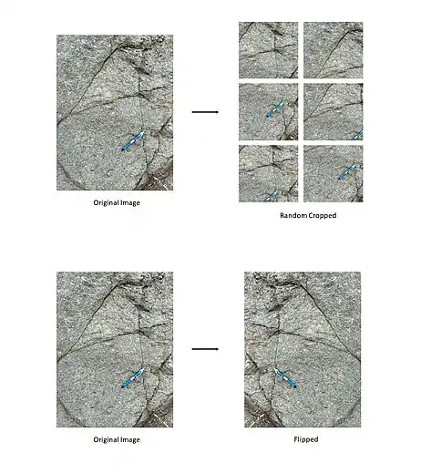
In the preparation of the dataset for the recognition of rock fractures, data augmentation was carried out. This technique is commonly used for increasing the training dataset size. Although the randomly cropped samples and the flipping samples come from the same image, the processed samples are unique to the learning. This technique can prevent the problem of data scarcity and the overfitting problem of the model.
Discontinuity analyses
Discontinuities such as a fault plane, bedding plane etc have important implications in engineering.[34] Rock fractures can be recognized automatically by machine learning through photogrammetric analysis even with the presence of interfering objects, for example, foliation, rod-shaped vegetation, etc.[35] In machine training for classifying images, data augmentation is a common practice to avoid overfitting and increase the training dataset.[35] For example, in a research of recognizing rock fractures, 68 images for training and 23 images for the testing dataset were prepared by random splitting.[35] Data augmentation was then carried out and the training dataset was increased to 8704 images by flip and random crop.[35] The approach was able to recognize the rock fractures accurately in most cases.[35] The Negative Prediction Value (NPV) and the Specificity were over 0.99.[35] This demonstrated the robustness of discontinuity analyses with machine learning.
| Objective | Input dataset | Location | Machine Learning Algorithms (MLAs) | Performance |
|---|---|---|---|---|
| Recognition of Rock Fractures[35] | Rock images collected in field survey | Gwanak Mountain and Bukhan Mountain,
Seoul, Korea and Jeongseon-gun, Gangwon-do, Korea |
Convolutional Neural Network (CNN) | The approach was able to recognize the rock fractures accurately in most cases. The Negative Prediction Value (NPV) and the Specificity are over 0.99. |
Carbon dioxide leakage detection
Quantifying carbon dioxide leakage from a geologic sequestration site has been gaining increasing attention as the public is interested in whether carbon dioxide is stored underground safely and effectively.[36] A geologic sequestration site is to capture greenhouse gas and bury deep underground in the geological formations. Carbon dioxide leakage from a geologic sequestration site can be detected indirectly by planet stress response with the aid of remote sensing and an unsupervised clustering algorithm (Iterative Self-Organizing Data Analysis Technique (ISODATA) method).[37] The increase in soil CO2 concentration causes a stress response for the plants by inhibiting plant respiration as oxygen is displaced away by carbon dioxide.[38] The stress signal by the vegetation can be detected with the Red Edge Index (REI).[38] The hyperspectral images are processed by the unsupervised algorithm clustering pixels with similar plant responses.[38] The hyperspectral information in areas with known CO2 leakage was extracted so that areas with CO2 leakage can be matched with the clustered pixels with spectral anomalies.[38] Although the approach can identify CO2 leakage efficiently, there are some limitations that require further study.[38] The Red Edge Index (REI) may not be accurate due to reasons like higher chlorophyll absorption, variation in vegetation, and shadowing effects therefore some stressed pixels were incorrectly identified as healthy pixels.[38] Seasonality, groundwater table height may also affect the stress response to CO2 of the vegetation.[38]
| Objective | Input dataset | Location | Machine Learning Algorithms (MLAs) | Performance |
|---|---|---|---|---|
| Detection of CO2 leak from a geologic sequestration site[37] | Aerial hyperspectral imagery | The Zero Emissions Research and Technology (ZERT),
US |
Iterative Self-Organizing Data Analysis Technique (ISODATA) method | The approach was able to detect areas with CO2 leak,s however other factors like the growing seasons of the vegetation also interfere with the results. |
Quantification of water inflow
The Rock Mass Rating (RMR) System[39] a world-wide adopted rock mass classification system by geomechanical means with the input of six parameters. The amount of water inflow is one of the inputs of the classification scheme, representing the groundwater condition. Quantification of the water inflow in the faces of a rock tunnel was traditionally carried out by visual observation in the field, which is labour and time consuming with safety concerns.[40] Machine learning can determine the water inflow by analyzing images taken in the construction site.[40] The classification of the approach mostly follows the RMR system but combining damp and wet state as its difficult to distinguish only by visual inspection.[40][39] The images were classified into the non-damage state, wet state, dripping state, flowing state and gushing state.[40] The accuracy of classifying the images was about 90%.[40]
| Objective | Input dataset | Location | Machine Learning Algorithms (MLAs) | Performance |
|---|---|---|---|---|
| Quantification of water inflow in rock tunnel faces[40] | Images of water inflow | - | Convolutional Neural Network (CNN) | The approach achieved an average accuracy of 93.01%. |
Classification
Soil classification
The most popular cost-effective method for soil investigation method is by Cone Penetration Testing (CPT).[41] The test is carried out by pushing a metallic cone through the soil and the force required to push at a constant rate is recorded as a quasi-continuous log.[4] Machine learning can classify soil with the input of Cone Penetration Test log data.[4] In an attempt to classify with machine learning, there are two parts of tasks required to analyse the data, which are the segmentation and classification parts.[4] The segmentation part can be carried out with the Constraint Clustering and Classification (CONCC) algorithm to split a single series data into segments.[4] The classification part can be carried out by Decision Trees (DT), Artificial Neural Network (ANN), or Support Vector Machine (SVM).[4] While comparing the three algorithms, it is demonstrated that the Artificial Neural Network (ANN) performed the best in classifying humous clay and peat, while the Decision Trees performed the best in classifying clayey peat.[4] The classification by this method is able to reach very high accuracy, even for the most complex problem, its accuracy was 83%, and the incorrectly classified class was a geologically neighbouring one.[4] Considering the fact that such accuracy is sufficient for most experts, therefore the accuracy of such approach can be regarded as 100%.[4]
| Objective | Input dataset | Location | Machine Learning Algorithms (MLAs) | Performance |
|---|---|---|---|---|
| Soil classification[4] | Cone Penetration Test (CPT) logs | - | Decision Trees,
Artificial Neural Network (ANN), Support Vector Machine |
The Artificial Neural Network (ANN) outperformed the others in classifying humous clay and peat, while the Decision Trees outperformed the others in classifying clayey peat. Support Vector Machine gave the poorest performance among the three. |
Geological structure classification
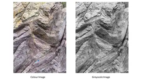
Exposed geological structures like anticline, ripple marks, xenolith, scratch, ptygmatic folds, fault, concretion, mudcracks, gneissose, boudin, basalt columns and dike can be identified automatically with a deep learning model.[20] Research demonstrated that Three-layer Convolutional Neural Network (CNN) and Transfer Learning have great accuracy of about 80% and 90% respectively, while others like K-nearest neighbors (KNN), Artificial Neural Network (ANN) and Extreme Gradient Boosting (XGBoost) have low accuracies, ranges from 10% - 30%.[20] The grayscale images and colour images were both tested, and the accuracies difference is little, inferring that colour is not very important in identifying geological structures.[20]
| Objective | Input dataset | Location | Machine Learning Algorithms (MLAs) | Performance |
|---|---|---|---|---|
| Geological structures classification[20] | Images of geological structures | - | K nearest neighbors (KNN),
Artificial Neural Network (ANN), Extreme Gradient Boosting (XGBoost), Three-layer Convolutional Neural Network (CNN), Transfer Learning |
Three-layer Convolutional Neural Network (CNN) and Transfer Learning reached accuracies up to about 80% and 90% respectively, while others were relatively low, ranges from about 10% to 30%. |
Forecast and predictions
Earthquake early warning systems and forecasting
Earthquake early warning systems are often vulnerable to local impulsive noise, therefore giving out false alerts.[42] False alerts can be eliminated by discriminating the earthquake waveforms from noise signals with the aid of machine learning methods. The method consists of two parts, the first part is unsupervised learning with Generative Adversarial Network (GAN) to learn and extract features of first arrival P-waves, and Random Forest to discriminate P-waves. The approach achieved 99.2% in recognizing P-waves and can avoid false triggers by noise signals with 98.4% accuracy.[42]
Laboratory earthquakes are produced in a laboratory setting to mimic real-world earthquakes. With the help of machine learning, the patterns of acoustical signals as precursors for earthquakes can be identified without the need of manually searching. Predicting the time remaining before failure was demonstrated in a research with continuous acoustic time series data recorded from a fault. The algorithm applied was Random Forest trained with about 10 slip events and performed excellently in predicting the remaining time to failure. It identified acoustic signals to predict failures, and one of them was previously unidentified. Although this laboratory earthquake produced is not as complex as that of earth, this makes important progress that guides further earthquake prediction work in the future.[43]
| Objective | Input dataset | Location | Machine Learning Algorithms (MLAs) | Performance |
|---|---|---|---|---|
| Discriminating earthquake waveforms[42] | Earthquake dataset | Southern California and Japan | Generative Adversarial Network (GAN),
Random Forest |
The approach can recognise P waves with 99.2% accuracy and avoid false triggers by noise signals with 98.4% accuracy. |
| Predicting time remaining for next earthquake[43] | Continuous acoustic time series data | - | Random Forest | The R2 value of the prediction reached 0.89, which demonstrated excellent performance. |
Streamflow discharge prediction
Real-time streamflow data is integral for decision making, for example, evacuations, regulation of reservoir water levels during a flooding event.[44] Streamflow data can be estimated by information provided by streamgages which measures the water level of a river. However, water and debris from a flooding event may damage streamgages and essential real-time data will be missing. The ability of machine learning to infer missing data[10] enables it to predict streamflow with both historical streamgages data and real-time data. SHEM is a model that refers to Streamflow Hydrology Estimate using Machine Learning[45] that can serve the purpose. To verify its accuracies, the prediction result was compared with the actual recorded data and the accuracies were found to be between 0.78 to 0.99.
| Objective | Input dataset | Location | Machine Learning Algorithms (MLAs) | Performance |
|---|---|---|---|---|
| Streamflow Estimate with data missing[45] | Streamgage data from NWIS-Web | Four diverse watersheds in Idaho and Washington,
US |
Random Forests | The estimates correlated well to the historical data of the discharges. The accuracy ranges from 0.78 to 0.99. |
Challenge
Inadequate training data
An adequate amount of training and validation data is required for machine learning.[10] However, some very useful products like satellite remote sensing data only have decades of data since the 1970s. If one is interested in the yearly data, then only less than 50 samples are available.[46] Such amount of data may not be adequate. In a study of automatic classification of geological structures, the weakness of the model is the small training dataset, even though with the help of data augmentation to increase the size of the dataset.[20] Another study of predicting streamflow found that the accuracies depend on the availability of sufficient historical data, therefore sufficient training data determine the performance of machine learning.[45] Inadequate training data may lead to a problem called overfitting. Overfitting causes inaccuracies in machine learning[47] as the model learns about the noise and undesired details.
Limited by data input
Machine learning cannot carry out some of the tasks as a human does easily. For example, in the quantification of water inflow in rock tunnel faces by images for Rock Mass Rating system (RMR),[40] the damp and the wet state was not classified by machine learning because discriminating the two only by visual inspection is not possible. In some tasks, machine learning may not able to fully substitute manual work by a human.
Black-box operation

In a black-box operation, a user only know about the input and output but not the process. Artificial Neural Network (ANN) is an example of a black-box operation. The user has no way to understand the logic of the hidden layers.
In many machine learning algorithms, for example, Artificial Neural Network (ANN), it is considered as 'black box' approach as clear relationships and descriptions of how the results are generated in the hidden layers are unknown.[48] 'White-box' approach such as decision tree can reveal the algorithm details to the users.[49] If one wants to investigate the relationships, such 'black-box' approaches are not suitable. However, the performances of 'black-box' algorithms are usually better.[50]
References
- ↑ Mueller, J. P., & Massaron, L. (2021). Machine learning for dummies. John Wiley & Sons.
- ↑ Resources., National Academies Press (U.S.) National Research Council (U.S.). Commission on Geosciences, Environment, and (2001). Basic research opportunities in earth science. National Academies Press. OCLC 439353646.
{{cite book}}: CS1 maint: multiple names: authors list (link) - ↑ Miall, A.D. (December 1995). "The blue planet: An introduction to earth system science". Earth-Science Reviews. 39 (3–4): 269–271. doi:10.1016/0012-8252(95)90023-3. ISSN 0012-8252.
- 1 2 3 4 5 6 7 8 9 10 11 12 Bhattacharya, B.; Solomatine, D.P. (March 2006). "Machine learning in soil classification". Neural Networks. 19 (2): 186–195. doi:10.1016/j.neunet.2006.01.005. ISSN 0893-6080. PMID 16530382. S2CID 14421859.
- 1 2 3 4 5 Sang, Xuejia; Xue, Linfu; Ran, Xiangjin; Li, Xiaoshun; Liu, Jiwen; Liu, Zeyu (2020-02-05). "Intelligent High-Resolution Geological Mapping Based on SLIC-CNN". ISPRS International Journal of Geo-Information. 9 (2): 99. Bibcode:2020IJGI....9...99S. doi:10.3390/ijgi9020099. ISSN 2220-9964.
- ↑ Si, Lei; Xiong, Xiangxiang; Wang, Zhongbin; Tan, Chao (2020-03-14). "A Deep Convolutional Neural Network Model for Intelligent Discrimination between Coal and Rocks in Coal Mining Face". Mathematical Problems in Engineering. 2020: 1–12. doi:10.1155/2020/2616510. ISSN 1024-123X.
- 1 2 3 4 5 6 7 8 9 10 11 12 Marjanović, Miloš; Kovačević, Miloš; Bajat, Branislav; Voženílek, Vít (November 2011). "Landslide susceptibility assessment using SVM machine learning algorithm". Engineering Geology. 123 (3): 225–234. Bibcode:2011EngGe.123..225M. doi:10.1016/j.enggeo.2011.09.006. ISSN 0013-7952.
- ↑ Merembayev, Timur; Yunussov, Rassul; Yedilkhan, Amirgaliyev (November 2018). "Machine Learning Algorithms for Classification Geology Data from Well Logging". 2018 14th International Conference on Electronics Computer and Computation (ICECCO). IEEE. pp. 206–212. doi:10.1109/icecco.2018.8634775. ISBN 978-1-7281-0132-3. S2CID 59620103.
- ↑ De'ath, Glenn; Fabricius, Katharina E. (November 2000). "Classification and Regression Trees: A Powerful Yet Simple Technique for Ecological Data Analysis". Ecology. 81 (11): 3178–3192. doi:10.1890/0012-9658(2000)081[3178:cartap]2.0.co;2. ISSN 0012-9658.
- 1 2 3 4 5 Thessen, Anne (2016-06-27). "Adoption of Machine Learning Techniques in Ecology and Earth Science". One Ecosystem. 1: e8621. doi:10.3897/oneeco.1.e8621. ISSN 2367-8194.
- ↑ Zhao, Kaiguang; Popescu, Sorin; Meng, Xuelian; Pang, Yong; Agca, Muge (August 2011). "Characterizing forest canopy structure with lidar composite metrics and machine learning". Remote Sensing of Environment. 115 (8): 1978–1996. Bibcode:2011RSEnv.115.1978Z. doi:10.1016/j.rse.2011.04.001. ISSN 0034-4257.
- ↑ LAWLER, JOSHUA J.; WHITE, DENIS; NEILSON, RONALD P.; BLAUSTEIN, ANDREW R. (2006-06-26). "Predicting climate-induced range shifts: model differences and model reliability". Global Change Biology. 12 (8): 1568–1584. Bibcode:2006GCBio..12.1568L. CiteSeerX 10.1.1.582.9206. doi:10.1111/j.1365-2486.2006.01191.x. ISSN 1354-1013. S2CID 37416127.
- ↑ Tartakovsky, Daniel M. (2004). "Delineation of geologic facies with statistical learning theory". Geophysical Research Letters. 31 (18). Bibcode:2004GeoRL..3118502T. CiteSeerX 10.1.1.146.5147. doi:10.1029/2004gl020864. ISSN 0094-8276. S2CID 16256805.
- ↑ Hurtt, George C.; Dubayah, Ralph; Drake, Jason; Moorcroft, Paul R.; Pacala, Stephen W.; Blair, J. Bryan; Fearon, Matthew G. (June 2004). "Beyond Potential Vegetation: Combining Lidar Data and a Height-Structured Model for Carbon Studies". Ecological Applications. 14 (3): 873–883. doi:10.1890/02-5317. ISSN 1051-0761.
- ↑ Lawler, Joshua J.; White, Denis; Neilson, RONALD P.; Blaustein, Andrew R. (2006-06-26). "Predicting climate-induced range shifts: model differences and model reliability". Global Change Biology. 12 (8): 1568–1584. Bibcode:2006GCBio..12.1568L. CiteSeerX 10.1.1.582.9206. doi:10.1111/j.1365-2486.2006.01191.x. ISSN 1354-1013. S2CID 37416127.
- ↑ Akpokodje, E. G. (June 1979). "The importance of engineering geological mapping in the development of the Niger delta basin". Bulletin of the International Association of Engineering Geology. 19 (1): 101–108. doi:10.1007/bf02600459. ISSN 1435-9529. S2CID 129112606.
- 1 2 3 Costa, Iago; Tavares, Felipe; Oliveira, Junny (April 2019). "Predictive lithological mapping through machine learning methods: a case study in the Cinzento Lineament, Carajás Province, Brazil". Journal of the Geological Survey of Brazil. 2 (1): 26–36. doi:10.29396/jgsb.2019.v2.n1.3. ISSN 2595-1939. S2CID 134822423.
- 1 2 3 4 Latifovic, Rasim; Pouliot, Darren; Campbell, Janet (2018-02-16). "Assessment of Convolution Neural Networks for Surficial Geology Mapping in the South Rae Geological Region, Northwest Territories, Canada". Remote Sensing. 10 (2): 307. Bibcode:2018RemS...10..307L. doi:10.3390/rs10020307. ISSN 2072-4292.
- 1 2 3 4 Culverhouse, PF; Williams, R; Reguera, B; Herry, V; González-Gil, S (2003). "Do experts make mistakes? A comparison of human and machine identification of dinoflagellates". Marine Ecology Progress Series. 247: 17–25. Bibcode:2003MEPS..247...17C. doi:10.3354/meps247017. ISSN 0171-8630.
- 1 2 3 4 5 6 Zhang, Ye; Wang, Gang; Li, Mingchao; Han, Shuai (2018-12-04). "Automated Classification Analysis of Geological Structures Based on Images Data and Deep Learning Model". Applied Sciences. 8 (12): 2493. doi:10.3390/app8122493. ISSN 2076-3417.
- 1 2 Loyola-Gonzalez, Octavio (2019). "Black-Box vs. White-Box: Understanding Their Advantages and Weaknesses From a Practical Point of View". IEEE Access. 7: 154096–154113. doi:10.1109/ACCESS.2019.2949286. ISSN 2169-3536. S2CID 207831043.
- 1 2 3 4 Kumar, Chandan; Chatterjee, Snehamoy; Oommen, Thomas; Guha, Arindam (April 2020). "Automated lithological mapping by integrating spectral enhancement techniques and machine learning algorithms using AVIRIS-NG hyperspectral data in Gold-bearing granite-greenstone rocks in Hutti, India". International Journal of Applied Earth Observation and Geoinformation. 86: 102006. Bibcode:2020IJAEO..8602006K. doi:10.1016/j.jag.2019.102006. ISSN 0303-2434. S2CID 210040191.
- ↑ #algorithm gallery
- 1 2 Haykin, Simon S. (2009). Neural Networks and Learning Machines. Prentice Hall. ISBN 978-0-13-147139-9.
- 1 2 Harvey, A. S.; Fotopoulos, G. (2016-06-23). "Geological Mapping Using Machine Learning Algorithms". ISPRS - International Archives of the Photogrammetry, Remote Sensing and Spatial Information Sciences. XLI-B8: 423–430. doi:10.5194/isprsarchives-xli-b8-423-2016. ISSN 2194-9034.
- ↑ Mattikalli, N (January 1997). "Soil color modeling for the visible and near-infrared bands of Landsat sensors using laboratory spectral measurements". Remote Sensing of Environment. 59 (1): 14–28. Bibcode:1997RSEnv..59...14M. doi:10.1016/s0034-4257(96)00075-2. ISSN 0034-4257.
- ↑ Radford, D. D., Cracknell, M. J., Roach, M. J., & Cumming, G. V. (2018). Geological mapping in western Tasmania using radar and random forests. IEEE Journal of Selected Topics in Applied Earth Observations and Remote Sensing, 11(9), 3075-3087.
- ↑ Wang, Y., Ksienzyk, A. K., Liu, M., & Brönner, M. (2021). Multigeophysical data integration using cluster analysis: assisting geological mapping in Trøndelag, Mid-Norway. Geophysical Journal International, 225(2), 1142-1157.
- ↑ "Phillips River landslide hazard mapping project", Landslide Risk Management, CRC Press, pp. 457–466, 2005-06-30, doi:10.1201/9781439833711-28, ISBN 9780429151354, retrieved 2021-11-12
- 1 2 Chauhan, S., Sharma, M., Arora, M. K., & Gupta, N. K. (2010). Landslide susceptibility zonation through ratings derived from artificial neural network. International Journal of Applied Earth Observation and Geoinformation, 12(5), 340-350.
- 1 2 Biswajeet, Pradhan; Saro, Lee (November 2007). "Utilization of Optical Remote Sensing Data and GIS Tools for Regional Landslide Hazard Analysis Using an Artificial Neural Network Model". Earth Science Frontiers. 14 (6): 143–151. Bibcode:2007ESF....14..143B. doi:10.1016/s1872-5791(08)60008-1. ISSN 1872-5791.
- ↑ Dou, Jie; Yamagishi, Hiromitsu; Pourghasemi, Hamid Reza; Yunus, Ali P.; Song, Xuan; Xu, Yueren; Zhu, Zhongfan (2015-05-19). "An integrated artificial neural network model for the landslide susceptibility assessment of Osado Island, Japan". Natural Hazards. 78 (3): 1749–1776. doi:10.1007/s11069-015-1799-2. ISSN 0921-030X. S2CID 51960414.
- 1 2 Kawabata, Daisaku; Bandibas, Joel (December 2009). "Landslide susceptibility mapping using geological data, a DEM from ASTER images and an Artificial Neural Network (ANN)". Geomorphology. 113 (1–2): 97–109. Bibcode:2009Geomo.113...97K. doi:10.1016/j.geomorph.2009.06.006. ISSN 0169-555X.
- ↑ "International society for rock mechanics commission on standardization of laboratory and field tests". International Journal of Rock Mechanics and Mining Sciences & Geomechanics Abstracts. 15 (6): 319–368. December 1978. doi:10.1016/0148-9062(78)91472-9. ISSN 0148-9062.
- 1 2 3 4 5 6 7 Byun, Hoon; Kim, Jineon; Yoon, Dongyoung; Kang, Il-Seok; Song, Jae-Joon (2021-07-08). "A deep convolutional neural network for rock fracture image segmentation". Earth Science Informatics. 14 (4): 1937–1951. Bibcode:2021EScIn..14.1937B. doi:10.1007/s12145-021-00650-1. ISSN 1865-0473. S2CID 235762914.
- ↑ Repasky, Kevin (2014-03-31). Development and Deployment of a Compact Eye-Safe Scanning Differential absorption Lidar (DIAL) for Spatial Mapping of Carbon Dioxide for Monitoring/Verification/Accounting at Geologic Sequestration Sites (Report). doi:10.2172/1155030. OSTI 1155030.
- 1 2 Bellante, G.J.; Powell, S.L.; Lawrence, R.L.; Repasky, K.S.; Dougher, T.A.O. (March 2013). "Aerial detection of a simulated CO2 leak from a geologic sequestration site using hyperspectral imagery". International Journal of Greenhouse Gas Control. 13: 124–137. Bibcode:2013IJGGC..13..124B. doi:10.1016/j.ijggc.2012.11.034. ISSN 1750-5836.
- 1 2 3 4 5 6 7 BATESON, L; VELLICO, M; BEAUBIEN, S; PEARCE, J; ANNUNZIATELLIS, A; CIOTOLI, G; COREN, F; LOMBARDI, S; MARSH, S (July 2008). "The application of remote-sensing techniques to monitor CO2-storage sites for surface leakage: Method development and testing at Latera (Italy) where naturally produced CO2 is leaking to the atmosphere". International Journal of Greenhouse Gas Control. 2 (3): 388–400. Bibcode:2008IJGGC...2..388B. doi:10.1016/j.ijggc.2007.12.005. ISSN 1750-5836.
- 1 2 Bieniawski, Z. T. (1988), "The Rock Mass Rating (RMR) System (Geomechanics Classification) in Engineering Practice", Rock Classification Systems for Engineering Purposes, West Conshohocken, PA: ASTM International, pp. 17–17–18, doi:10.1520/stp48461s, ISBN 978-0-8031-6663-9, retrieved 2021-11-12
- 1 2 3 4 5 6 7 Chen, Jiayao; Zhou, Mingliang; Zhang, Dongming; Huang, Hongwei; Zhang, Fengshou (March 2021). "Quantification of water inflow in rock tunnel faces via convolutional neural network approach". Automation in Construction. 123: 103526. doi:10.1016/j.autcon.2020.103526. ISSN 0926-5805. S2CID 233849934.
- ↑ Coerts, Alfred (1996). Analysis of static cone penetration test data for subsurface modelling : a methodology. Koninklijk Nederlands Aardrijkskundig Genootschap/Faculteit Ruimtelijke Wetenschappen Universiteit Utrecht. ISBN 90-6809-230-8. OCLC 37725852.
- 1 2 3 Li, Zefeng; Meier, Men-Andrin; Hauksson, Egill; Zhan, Zhongwen; Andrews, Jennifer (2018-05-28). "Machine Learning Seismic Wave Discrimination: Application to Earthquake Early Warning". Geophysical Research Letters. 45 (10): 4773–4779. Bibcode:2018GeoRL..45.4773L. doi:10.1029/2018gl077870. ISSN 0094-8276. S2CID 54926314.
- 1 2 Rouet-Leduc, Bertrand; Hulbert, Claudia; Lubbers, Nicholas; Barros, Kipton; Humphreys, Colin J.; Johnson, Paul A. (2017-09-22). "Machine Learning Predicts Laboratory Earthquakes". Geophysical Research Letters. 44 (18): 9276–9282. arXiv:1702.05774. Bibcode:2017GeoRL..44.9276R. doi:10.1002/2017gl074677. ISSN 0094-8276. S2CID 118842086.
- ↑ Kirchner, James W. (March 2006). "Getting the right answers for the right reasons: Linking measurements, analyses, and models to advance the science of hydrology". Water Resources Research. 42 (3). Bibcode:2006WRR....42.3S04K. doi:10.1029/2005wr004362. ISSN 0043-1397. S2CID 2089939.
- 1 2 3 Petty, T.R.; Dhingra, P. (2017-08-08). "Streamflow Hydrology Estimate Using Machine Learning (SHEM)". JAWRA Journal of the American Water Resources Association. 54 (1): 55–68. doi:10.1111/1752-1688.12555. ISSN 1093-474X. S2CID 135100027.
- ↑ Karpatne, Anuj; Ebert-Uphoff, Imme; Ravela, Sai; Babaie, Hassan Ali; Kumar, Vipin (2019-08-01). "Machine Learning for the Geosciences: Challenges and Opportunities". IEEE Transactions on Knowledge and Data Engineering. 31 (8): 1544–1554. arXiv:1711.04708. doi:10.1109/tkde.2018.2861006. ISSN 1041-4347. S2CID 42476116.
- ↑ Farrar, Donald E.; Glauber, Robert R. (February 1967). "Multicollinearity in Regression Analysis: The Problem Revisited". The Review of Economics and Statistics. 49 (1): 92. doi:10.2307/1937887. hdl:1721.1/48530. ISSN 0034-6535. JSTOR 1937887.
- ↑ Taghizadeh-Mehrjardi, R.; Nabiollahi, K.; Kerry, R. (March 2016). "Digital mapping of soil organic carbon at multiple depths using different data mining techniques in Baneh region, Iran". Geoderma. 266: 98–110. Bibcode:2016Geode.266...98T. doi:10.1016/j.geoderma.2015.12.003. ISSN 0016-7061.
- ↑ Delibasic, Boris; Vukicevic, Milan; Jovanovic, Milos; Suknovic, Milija (August 2013). "White-Box or Black-Box Decision Tree Algorithms: Which to Use in Education?". IEEE Transactions on Education. 56 (3): 287–291. Bibcode:2013ITEdu..56..287D. doi:10.1109/te.2012.2217342. ISSN 0018-9359. S2CID 11792899.
- ↑ Merghadi, Abdelaziz; Yunus, Ali P.; Dou, Jie; Whiteley, Jim; ThaiPham, Binh; Bui, Dieu Tien; Avtar, Ram; Abderrahmane, Boumezbeur (August 2020). "Machine learning methods for landslide susceptibility studies: A comparative overview of algorithm performance". Earth-Science Reviews. 207: 103225. Bibcode:2020ESRv..20703225M. doi:10.1016/j.earscirev.2020.103225. ISSN 0012-8252. S2CID 225816933.