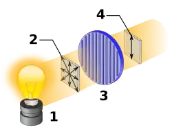
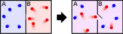
從白熾燈 (1)發射出的光子處於完全隨機偏振混合態(2),密度矩陣為
[
0.5
0
0
0.5
]
{\displaystyle {\begin{bmatrix}0.5&0\\0&0.5\\\end{bmatrix}}}
。
[
1
0
0
0
]
{\displaystyle {\begin{bmatrix}1&0\\0&0\\\end{bmatrix}}}
。 在量子力學 裏,密度算符 (英語:density operator 密度矩陣 (英語:density matrix
|
ψ
⟩
{\displaystyle |\psi \rangle }
量子態 ,混合態則是由幾種純態依照統計機率 組成的量子態。假設一個量子系統處於純態
|
ψ
1
⟩
{\displaystyle |\psi _{1}\rangle }
|
ψ
2
⟩
{\displaystyle |\psi _{2}\rangle }
|
ψ
3
⟩
{\displaystyle |\psi _{3}\rangle }
w
1
{\displaystyle w_{1}}
w
2
{\displaystyle w_{2}}
w
3
{\displaystyle w_{3}}
ρ
{\displaystyle \rho }
ρ
=
∑
i
w
i
|
ψ
i
⟩
⟨
ψ
i
|
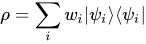
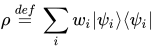
{\displaystyle {\rho }=\sum _{i}w_{i}|\psi _{i}\rangle \langle \psi _{i}|}
注意到所有機率的總和為1:
∑
i
w
i
=
1
{\displaystyle \sum _{i}w_{i}=1}
假設
{
|
b
i
⟩
,
i
=
1
,
2
,
3
,
…
,
n
}
{\displaystyle \{|b_{i}\rangle ,\quad i=1,2,3,\dots ,n\}}
ϱ
{\displaystyle \varrho }
ϱ
i
j
{\displaystyle \varrho _{ij}}
ϱ
i
j
=
⟨
b
i
|
ρ
|
b
j
⟩
=
∑
k
w
k
⟨
b
i
|
ψ
k
⟩
⟨
ψ
k
|
b
j
⟩
{\displaystyle \varrho _{ij}=\langle b_{i}|\rho |b_{j}\rangle =\sum _{k}w_{k}\langle b_{i}|\psi _{k}\rangle \langle \psi _{k}|b_{j}\rangle }
對於這量子系統,可觀察量
A
{\displaystyle A}
期望值 為
⟨
A
⟩
=
∑
i
w
i
⟨
ψ
i
|
A
|
ψ
i
⟩
=
∑
i
⟨
b
i
|
ρ
A
|
b
i
⟩
=
tr
(
ρ
A
)
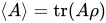
{\displaystyle \langle A\rangle =\sum _{i}w_{i}\langle \psi _{i}|{A}|\psi _{i}\rangle =\sum _{i}\langle b_{i}|{\rho }{A}|b_{i}\rangle =\operatorname {tr} ({\rho }{A})}
是可觀察量
A
{\displaystyle A}
⟨
ψ
i
|
A
|
ψ
i
⟩
{\displaystyle \langle \psi _{i}|{A}|\psi _{i}\rangle }
權值
w
i
{\displaystyle w_{i}}
混合態量子系統出現的案例包括,處於熱力學平衡 或化學平衡 的系統、製備歷史不確定或隨機 變化的系統(因此不知道到底系統處於哪個純態)。假設量子系統處於由幾個糾纏 在一起的子系統所組成的純態,則雖然整個系統處於純態,每一個子系統仍舊可能處於混合態。在量子退相干 理論裏,密度算符是重要理論工具。
密度算符是一種線性算符 ,是自伴算符、非負算符(英語:nonnegative operator )、跡數 為1的算符。關於密度算符的數學形式論是由約翰·馮·諾伊曼 與列夫·郎道 各自獨立於1927年給出。[ 1] [ 2] : 48–55 [ 3]
假設一個量子系統的量子態是純態,則這量子態可以用態向量表示為
|
ψ
⟩
{\displaystyle |\psi \rangle }
|
ψ
1
⟩
{\displaystyle |\psi _{1}\rangle }
|
ψ
2
⟩
{\displaystyle |\psi _{2}\rangle }
混合態與疊加態 的概念不同,幾種純態通過量子疊加所組成的疊加態仍舊是純態。例如,
(
|
ψ
1
⟩
+
|
ψ
2
⟩
)
/
2
{\displaystyle (|\psi _{1}\rangle +|\psi _{2}\rangle )/{\sqrt {2}}}
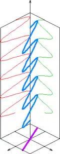
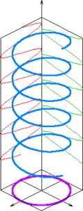
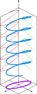
平面偏振(紫色)光波的電場(藍色)可以分解為兩個相互垂直的分量(紅色與綠色)。
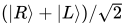
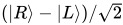
光子的兩種圓偏振態 ,右旋圓偏振態與左旋圓偏振態,分別以態向量
|
R
⟩
{\displaystyle |R\rangle }
|
L
⟩
{\displaystyle |L\rangle }
(
|
R
⟩
+
|
L
⟩
)
/
2
{\displaystyle (|R\rangle +|L\rangle )/{\sqrt {2}}}
(
|
R
⟩
−
|
L
⟩
)
/
2
{\displaystyle (|R\rangle -|L\rangle )/{\sqrt {2}}}
α
|
R
⟩
+
β
|
L
⟩
{\displaystyle \alpha |R\rangle +\beta |L\rangle }
α
{\displaystyle \alpha }
β
{\displaystyle \beta }
假若讓處於疊加態
(
|
R
⟩
+
|
L
⟩
)
/
2
{\displaystyle (|R\rangle +|L\rangle )/{\sqrt {2}}}
|
L
⟩
{\displaystyle |L\rangle }
|
R
⟩
{\displaystyle |R\rangle }
(
|
R
⟩
+
|
L
⟩
)
/
2
{\displaystyle (|R\rangle +|L\rangle )/{\sqrt {2}}}
|
R
⟩
{\displaystyle |R\rangle }
|
L
⟩
{\displaystyle |L\rangle }
|
R
⟩
{\displaystyle |R\rangle }
|
L
⟩
{\displaystyle |L\rangle }
(
|
R
⟩
+
|
L
⟩
)
/
2
{\displaystyle (|R\rangle +|L\rangle )/{\sqrt {2}}}
從白熾燈 發射出的光子是一種非偏振態 光子,不能用疊加態
α
|
R
⟩
+
β
|
L
⟩
{\displaystyle \alpha |R\rangle +\beta |L\rangle }
|
R
⟩
{\displaystyle |R\rangle }
|
L
⟩
{\displaystyle |L\rangle }
非偏振態光子的量子態不是純態,而是由幾種純態依照統計機率組成。它可以由50%右旋圓偏振態與50%左旋圓偏振態組成,或者,它可以由50%垂直偏振態與50%水平偏振態組成。這兩種組合無法做實驗辨識區分,因此它們被視為同樣的混合態。密度算符含有混合態的所有資料,足夠計算任何關於混合態的可測量性質。
混合態到底源自何處?試想非偏振態光子是怎樣製成的。一種方法是利用處於動力學平衡的系統,這系統擁有很多個微觀態(microstate),伴隨每一個微觀態都有其發生的機率(波茲曼因子),它們會因熱力學漲落(thermal fluctuation)從一個微觀態變換到另一個微觀態。熱力學隨機性可以解釋白熾燈怎樣發射非偏振光子。另一種方法是引入不確定性於系統的製備程序,例如,將光束通過表面粗糙的雙折射晶體 ,使得光束的不同部分獲得不同偏振。第三種方法應用EPR機制 ,有些放射性衰變會發射兩個光子朝著反方向移動離開,這糾纏系統的量子態為
(
|
R
,
L
⟩
+
|
L
,
R
⟩
)
/
2
{\displaystyle (|R,L\rangle +|L,R\rangle )/{\sqrt {2}}}
一般而言,混合態時常會出現於幾種純態的統計性混合(例如熱力學平衡)、製備程序的不確定性(例如光子可能移動於稍微不同路徑)、包含在糾纏系統內的子系統(例如EPR機制)。
假設一個量子系統的量子態是純態,則這量子態可以用態向量表示為
|
ψ
⟩
{\displaystyle |\psi \rangle }
[ 4] : 309–313
ρ
=
d
e
f
|
ψ
⟩
⟨
ψ
|
{\displaystyle \rho \ {\stackrel {def}{=}}\ |\psi \rangle \langle \psi |}
從密度算符的形式,可以推論密度算符是自伴算符:
ρ
†
=
(
|
ψ
⟩
⟨
ψ
|
)
†
=
|
ψ
⟩
⟨
ψ
|
=
ρ
{\displaystyle \rho ^{\dagger }=(|\psi \rangle \langle \psi |)^{\dagger }=|\psi \rangle \langle \psi |=\rho }
假設,物理量
A
{\displaystyle A}
本徵值 為
a
i
{\displaystyle a_{i}}
本徵態
|
a
i
⟩
,
i
=
1
,
2
,
3
,
⋯
,
n
{\displaystyle |a_{i}\rangle ,\quad i=1,\ 2,\ 3,\ \cdots ,n}
{
|
a
i
⟩
}
{\displaystyle \{|a_{i}\rangle \}}
A
{\displaystyle A}
a
i
{\displaystyle a_{i}}
P
(
a
i
)
{\displaystyle {\mathcal {P}}(a_{i})}
[ 5] : 96–99
P
(
a
i
)
=
d
e
f
|
⟨
a
i
|
ψ
⟩
|
2
=
⟨
a
i
|
ψ
⟩
⟨
ψ
|
a
i
⟩
=
∑
k
⟨
a
k
|
a
i
⟩
⟨
a
i
|
ψ
⟩
⟨
ψ
|
a
k
⟩
=
∑
k
⟨
a
k
|
Λ
(
a
i
)
ρ
|
a
k
⟩
=
tr
(
Λ
(
a
i
)
ρ
)
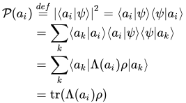
{\displaystyle {\begin{aligned}{\mathcal {P}}(a_{i})&\ {\stackrel {def}{=}}\ |\langle a_{i}|\psi \rangle |^{2}=\langle a_{i}|\psi \rangle \langle \psi |a_{i}\rangle \\&=\sum _{k}\langle a_{k}|a_{i}\rangle \langle a_{i}|\psi \rangle \langle \psi |a_{k}\rangle \\&=\sum _{k}\langle a_{k}|\Lambda (a_{i})\rho |a_{k}\rangle \\&={\hbox{tr}}(\Lambda (a_{i})\rho )\\\end{aligned}}}
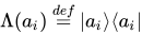
; 其中,
Λ
(
a
i
)
=
d
e
f
|
a
i
⟩
⟨
a
i
|
{\displaystyle \Lambda (a_{i})\ {\stackrel {def}{=}}\ |a_{i}\rangle \langle a_{i}|}
|
a
i
⟩
{\displaystyle |a_{i}\rangle }
投影算符 ,[ 註 1]
tr
(
)
{\displaystyle {\hbox{tr}}()}
跡數 。
做實驗測量可觀察量
A
{\displaystyle A}
期望值 為
⟨
A
⟩
=
d
e
f
∑
i
a
i
P
(
a
i
)
=
∑
i
a
i
⟨
a
i
|
ψ
⟩
⟨
ψ
|
a
i
⟩
=
∑
i
a
i
⟨
a
i
|
ρ
|
a
i
⟩
=
∑
i
⟨
a
i
|
A
ρ
|
a
i
⟩
=
tr
(
A
ρ
)
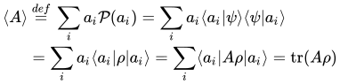
{\displaystyle {\begin{aligned}\langle A\rangle &\ {\stackrel {def}{=}}\ \sum _{i}a_{i}{\mathcal {P}}(a_{i})=\sum _{i}a_{i}\langle a_{i}|\psi \rangle \langle \psi |a_{i}\rangle \\&=\sum _{i}a_{i}\langle a_{i}|\rho |a_{i}\rangle =\sum _{i}\langle a_{i}|A\rho |a_{i}\rangle ={\hbox{tr}}(A\rho )\\\end{aligned}}}
。 這種可觀察量的期望值與跡數運算之間的關係稱為跡定則 (trace rule)。[ 6] : 36 [ 註 2] 線性 ,這是很優良的性質,這意味著機率公式與期望值公式也適用於幾個密度算符的線性組合。
由於
|
ψ
⟩
{\displaystyle |\psi \rangle }
tr
(
ρ
)
=
tr
(
|
ψ
⟩
⟨
ψ
|
)
=
∑
i
⟨
a
i
|
ψ
⟩
⟨
ψ
|
a
i
⟩
=
∑
i
⟨
ψ
|
a
i
⟩
⟨
a
i
|
ψ
⟩
=
⟨
ψ
|
ψ
⟩
=
1
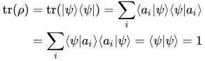
{\displaystyle {\begin{aligned}{\hbox{tr}}(\rho )&={\hbox{tr}}(|\psi \rangle \langle \psi |)=\sum _{i}\langle a_{i}|\psi \rangle \langle \psi |a_{i}\rangle \\&=\sum _{i}\langle \psi |a_{i}\rangle \langle a_{i}|\psi \rangle =\langle \psi |\psi \rangle =1\\\end{aligned}}}
。 對於任意歸一化量子態
ϕ
{\displaystyle \phi }
0
≤
⟨
ϕ
|
ρ
|
ϕ
⟩
=
⟨
ϕ
|
ψ
⟩
⟨
ψ
|
ϕ
⟩
=
|
⟨
ϕ
|
ψ
⟩
|
2
≤
1
{\displaystyle 0\leq \langle \phi |\rho |\phi \rangle =\langle \phi |\psi \rangle \langle \psi |\phi \rangle =|\langle \phi |\psi \rangle |^{2}\leq 1}
所以,密度算符是非負算符(nonnegative operator)。
將先前純態密度算符的定義式加以延伸,假設在一個量子系統處於純態
|
ψ
1
⟩
{\displaystyle |\psi _{1}\rangle }
|
ψ
2
⟩
{\displaystyle |\psi _{2}\rangle }
|
ψ
3
⟩
{\displaystyle |\psi _{3}\rangle }
w
1
{\displaystyle w_{1}}
w
2
{\displaystyle w_{2}}
w
3
{\displaystyle w_{3}}
ρ
{\displaystyle \rho }
[ 4] : 311–313
ρ
=
d
e
f
∑
i
w
i
|
ψ
i
⟩
⟨
ψ
i
|
{\displaystyle {\rho }\ {\stackrel {def}{=}}\ \sum _{i}w_{i}|\psi _{i}\rangle \langle \psi _{i}|}
每一個機率都是非負實值,所有機率的總和為1:
0
≤
w
i
≤
1
{\displaystyle 0\leq w_{i}\leq 1}
∑
i
w
i
=
1
{\displaystyle \sum _{i}w_{i}=1}
按照「無知詮釋」,這種量子系統確定是處於某個純態
ψ
i
{\displaystyle \psi _{i}}
[ 7] [ 註 3]
回想在純態段落裏,機率公式與期望值公式對於密度算符都具有線性 ,這意味著對於混合態的密度算符,這些公式也都適用。加以延伸後的密度算符,也具有先前純態的密度算符所擁有的性質:
密度算符是自伴算符:
ρ
=
ρ
†
{\displaystyle \rho =\rho ^{\dagger }}
密度算符的跡數為1:
tr
(
ρ
)
=
1
{\displaystyle {\hbox{tr}}(\rho )=1}
對可觀察量
A
{\displaystyle A}
a
i
{\displaystyle a_{i}}
P
(
a
i
)
=
tr
(
Λ
(
a
i
)
ρ
)
{\displaystyle {\mathcal {P}}(a_{i})={\hbox{tr}}(\Lambda (a_{i})\rho )}
做實驗測量可觀察量
A
{\displaystyle A}
期望值 為
⟨
A
⟩
=
tr
(
A
ρ
)
{\displaystyle \langle A\rangle ={\hbox{tr}}(A\rho )}
密度算符是非負算符:
0
≤
⟨
ϕ
|
ρ
|
ϕ
⟩
≤
1
{\displaystyle 0\leq \langle \phi |\rho |\phi \rangle \leq 1}
由於密度算符
ρ
{\displaystyle \rho }
ρ
=
∑
i
a
i
|
a
i
⟩
⟨
a
i
|
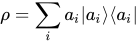
{\displaystyle \rho =\sum _{i}a_{i}|a_{i}\rangle \langle a_{i}|}
其中,
|
a
i
⟩
{\displaystyle |a_{i}\rangle }
本徵值 為
a
i
{\displaystyle a_{i}}
本徵態 ,所有
|
a
i
⟩
{\displaystyle |a_{i}\rangle }
按照自伴算符的定義,每一個本徵值
a
i
{\displaystyle a_{i}}
a
i
=
a
i
∗
{\displaystyle a_{i}=a_{i}^{*}}
由於密度算符
ρ
{\displaystyle \rho }
a
i
{\displaystyle a_{i}}
由於密度算符
ρ
{\displaystyle \rho }
∑
i
a
i
=
1
{\displaystyle \sum _{i}a_{i}=1}
給定一個量子系統,其所有可能的密度算符組成一個凸集 。假設
ρ
i
,
i
=
1
,
2
,
3
,
.
.
.
,
n
{\displaystyle \rho _{i},\quad i=1,2,3,...,n}
ρ
=
∑
i
c
i
ρ
i
{\displaystyle \rho =\sum _{i}c_{i}\rho _{i}}
0
≤
c
i
≤
1
{\displaystyle 0\leq c_{i}\leq 1}
∑
i
c
i
=
1
{\displaystyle \sum _{i}c_{i}=1}
[ 2] : 51
由於純態的密度算符定義式為[ 4] : 311–313
ρ
=
d
e
f
|
ψ
⟩
⟨
ψ
|
{\displaystyle \rho \ {\stackrel {def}{=}}\ |\psi \rangle \langle \psi |}
所以純態的密度算符具有特徵
ρ
2
=
ρ
{\displaystyle \rho ^{2}=\rho }
tr
(
ρ
2
)
=
tr
(
ρ
)
=
1
{\displaystyle {\hbox{tr}}(\rho ^{2})={\hbox{tr}}(\rho )=1}
否則,非純態的密度算符遵守關係式
tr
(
ρ
2
)
<
tr
(
ρ
)
=
1
{\displaystyle {\hbox{tr}}(\rho ^{2})<{\hbox{tr}}(\rho )=1}
另外,將純態的密度矩陣
ϱ
{\displaystyle \varrho }
[ 8] : 178–183
ϱ
=
[
0
0
0
⋯
0
0
1
0
⋯
0
0
0
0
⋯
0
⋮
⋮
⋮
⋱
⋮
0
0
0
⋯
0
]
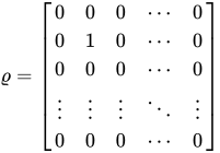
{\displaystyle \varrho ={\begin{bmatrix}0&0&0&\cdots &0\\0&1&0&\cdots &0\\0&0&0&\cdots &0\\\vdots &\vdots &\vdots &\ddots &\vdots \\0&0&0&\cdots &0\\\end{bmatrix}}}
。 量子態的純度
γ
{\displaystyle \gamma }
γ
=
tr
(
ρ
2
)
{\displaystyle \gamma ={\hbox{tr}}(\rho ^{2})}
純態的純度為1。處於N維希爾伯特空間、完全混合的混合態,其對角元素的數值為
1
/
N
{\displaystyle 1/N}
1
/
N
{\displaystyle 1/N}
[ 6] : 40–41
馮諾伊曼熵 是另一種描述量子態混合程度的量度。
位置是一種連續性 可觀察量,具有連續性本徵值譜,用這種可觀察量的連續性本徵態為基底,密度矩陣
ϱ
{\displaystyle \varrho }
x
′
{\displaystyle x'}
x
″
{\displaystyle x''}
[ 8] : 186
ϱ
(
x
′
,
x
″
)
=
∑
i
w
i
ψ
i
(
x
′
)
ψ
i
∗
(
x
″
)
{\displaystyle \varrho (x',x'')=\sum _{i}w_{i}\psi _{i}(x')\psi _{i}^{*}(x'')}
可觀察量
A
{\displaystyle A}
⟨
A
⟩
=
tr
(
A
ρ
)
=
∫
d
x
′
∫
d
x
″
⟨
x
′
|
A
|
x
″
⟩
⟨
x
″
|
ρ
|
x
′
⟩
{\displaystyle \langle A\rangle ={\hbox{tr}}(A\rho )=\int \mathrm {d} x'\int \mathrm {d} x''\langle x'|A|x''\rangle \langle x''|\rho |x'\rangle }
假設密度算符為
ρ
{\displaystyle \rho }
A
{\displaystyle A}
B
{\displaystyle B}
約化密度算符 (reduced density operator)
ρ
A
{\displaystyle \rho _{A}}
ρ
B
{\displaystyle \rho _{B}}
[ 4] : 120-125,128-129 [ 註 3]
ρ
A
=
tr
B
(
ρ
)
{\displaystyle \rho _{A}={\hbox{tr}}_{B}(\rho )}
ρ
B
=
tr
A
(
ρ
)
{\displaystyle \rho _{B}={\hbox{tr}}_{A}(\rho )}
其中,
tr
B
{\displaystyle {\hbox{tr}}_{B}}
tr
A
{\displaystyle {\hbox{tr}}_{A}}
B
{\displaystyle B}
A
{\displaystyle A}
偏跡數 (partial trace)。
這複合系統的兩個子系統之間沒有任何關聯(沒有任何量子關聯 或經典關聯),若且唯若
ρ
{\displaystyle \rho }
ρ
A
{\displaystyle \rho _{A}}
ρ
B
{\displaystyle \rho _{B}}
ρ
=
ρ
A
⊗
ρ
B
{\displaystyle \rho =\rho _{A}\otimes \rho _{B}}
約化密度算符最先由保羅·狄拉克 於1930年提出[ 9]
H
A
{\displaystyle H_{A}}
H
B
{\displaystyle H_{B}}
{
|
a
i
⟩
A
}
{\displaystyle \{|a_{i}\rangle _{A}\}}
{
|
b
j
⟩
B
}
{\displaystyle \{|b_{j}\rangle _{B}\}}
H
A
{\displaystyle H_{A}}
H
B
{\displaystyle H_{B}}
A
{\displaystyle A}
B
{\displaystyle B}
|
ψ
⟩
{\displaystyle |\psi \rangle }
密度算符
ρ
{\displaystyle \rho }
ρ
=
|
ψ
⟩
⟨
ψ
|
{\displaystyle \rho =|\psi \rangle \langle \psi |}
取密度算符
ρ
{\displaystyle \rho }
B
{\displaystyle B}
偏跡數 ,可以得到子系統
A
{\displaystyle A}
ρ
A
{\displaystyle \rho _{A}}
ρ
A
=
d
e
f
∑
j
⟨
b
j
|
B
(
|
ψ
⟩
⟨
ψ
|
)
|
b
j
⟩
B
=
tr
B
(
ρ
)
{\displaystyle \rho _{A}\ {\stackrel {\mathrm {def} }{=}}\ \sum _{j}\langle b_{j}|_{B}\left(|\psi \rangle \langle \psi |\right)|b_{j}\rangle _{B}={\hbox{tr}}_{B}(\rho )}
例如,糾纏態
|
ψ
⟩
A
B
=
(
|
0
⟩
A
⊗
|
1
⟩
B
−
|
1
⟩
A
⊗
|
0
⟩
B
)
/
2
{\displaystyle |\psi \rangle _{AB}=(|0\rangle _{A}\otimes |1\rangle _{B}-|1\rangle _{A}\otimes |0\rangle _{B})/{\sqrt {2}}}
A
{\displaystyle A}
ρ
A
{\displaystyle \rho _{A}}
ρ
A
=
1
2
(
|
0
⟩
A
⟨
0
|
A
+
|
1
⟩
A
⟨
1
|
A
)
{\displaystyle \rho _{A}={\frac {1}{2}}{\bigg (}|0\rangle _{A}\langle 0|_{A}+|1\rangle _{A}\langle 1|_{A}{\bigg )}}
如同預想,這公式演示出,子系統
A
{\displaystyle A}
ρ
A
{\displaystyle \rho _{A}}
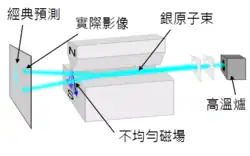
設定斯特恩-革拉赫實驗 儀器的磁場方向為z-軸,入射的銀原子束可以被分裂成兩道銀原子束,每一道銀原子束代表一種量子態,上旋
|
↑
⟩
{\displaystyle |\uparrow \rangle }
|
↓
⟩
{\displaystyle |\downarrow \rangle }
如右圖所示,使用z-軸方向的斯特恩-革拉赫實驗 儀器,可以將入射的銀原子束,依照自旋的z-分量
S
z
{\displaystyle S_{z}}
S
z
{\displaystyle S_{z}}
|
z
+
⟩
{\displaystyle |z+\rangle }
S
z
{\displaystyle S_{z}}
|
z
−
⟩
{\displaystyle |z-\rangle }
態向量:
|
z
+
⟩
=
[
1
0
]
{\displaystyle |z+\rangle ={\begin{bmatrix}1\\0\end{bmatrix}}}
密度矩陣:
ϱ
z
+
=
|
z
+
⟩
⟨
z
+
|
=
[
1
0
]
[
1
0
]
=
[
1
0
0
0
]
{\displaystyle \varrho _{z+}=|z+\rangle \langle z+|={\begin{bmatrix}1\\0\end{bmatrix}}{\begin{bmatrix}1&0\end{bmatrix}}={\begin{bmatrix}1&0\\0&0\end{bmatrix}}}
。 態向量:
|
z
−
⟩
=
[
0
1
]
{\displaystyle |z-\rangle ={\begin{bmatrix}0\\1\end{bmatrix}}}
密度矩陣:
ϱ
z
−
=
|
z
−
⟩
⟨
z
−
|
=
[
0
1
]
[
0
1
]
=
[
0
0
0
1
]
{\displaystyle \varrho _{z-}=|z-\rangle \langle z-|={\begin{bmatrix}0\\1\end{bmatrix}}{\begin{bmatrix}0&1\end{bmatrix}}={\begin{bmatrix}0&0\\0&1\end{bmatrix}}}
。
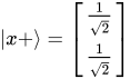
態向量:
|
x
+
⟩
=
[
1
2
1
2
]
{\displaystyle |x+\rangle ={\begin{bmatrix}{\frac {1}{\sqrt {2}}}\\{\frac {1}{\sqrt {2}}}\end{bmatrix}}}
密度矩陣:
ϱ
x
+
=
|
x
+
⟩
⟨
x
+
|
=
[
1
2
1
2
]
[
1
2
1
2
]
=
[
1
2
1
2
1
2
1
2
]
{\displaystyle \varrho _{x+}=|x+\rangle \langle x+|={\begin{bmatrix}{\frac {1}{\sqrt {2}}}\\{\frac {1}{\sqrt {2}}}\end{bmatrix}}{\begin{bmatrix}{\frac {1}{\sqrt {2}}}&{\frac {1}{\sqrt {2}}}\end{bmatrix}}={\begin{bmatrix}{\frac {1}{2}}&{\frac {1}{2}}\\{\frac {1}{2}}&{\frac {1}{2}}\end{bmatrix}}}
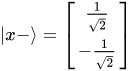
。 態向量:
|
x
−
⟩
=
[
1
2
−
1
2
]
{\displaystyle |x-\rangle ={\begin{bmatrix}{\frac {1}{\sqrt {2}}}\\-{\frac {1}{\sqrt {2}}}\end{bmatrix}}}
密度矩陣:
ϱ
x
−
=
|
x
−
⟩
⟨
x
−
|
=
[
1
2
−
1
2
]
[
1
2
−
1
2
]
=
[
1
2
−
1
2
−
1
2
1
2
]
{\displaystyle \varrho _{x-}=|x-\rangle \langle x-|={\begin{bmatrix}{\frac {1}{\sqrt {2}}}\\-{\frac {1}{\sqrt {2}}}\end{bmatrix}}{\begin{bmatrix}{\frac {1}{\sqrt {2}}}&-{\frac {1}{\sqrt {2}}}\end{bmatrix}}={\begin{bmatrix}{\frac {1}{2}}&-{\frac {1}{2}}\\-{\frac {1}{2}}&{\frac {1}{2}}\end{bmatrix}}}
。
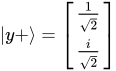
態向量:
|
y
+
⟩
=
[
1
2
i
2
]
{\displaystyle |y+\rangle ={\begin{bmatrix}{\frac {1}{\sqrt {2}}}\\{\frac {i}{\sqrt {2}}}\end{bmatrix}}}
密度矩陣:
ϱ
y
+
=
|
y
+
⟩
⟨
y
+
|
=
[
1
2
i
2
]
[
1
2
−
i
2
]
=
[
1
2
−
i
2
i
2
1
2
]
{\displaystyle \varrho _{y+}=|y+\rangle \langle y+|={\begin{bmatrix}{\frac {1}{\sqrt {2}}}\\{\frac {i}{\sqrt {2}}}\end{bmatrix}}{\begin{bmatrix}{\frac {1}{\sqrt {2}}}&-{\frac {i}{\sqrt {2}}}\end{bmatrix}}={\begin{bmatrix}{\frac {1}{2}}&-{\frac {i}{2}}\\{\frac {i}{2}}&{\frac {1}{2}}\end{bmatrix}}}
。 態向量:
|
y
−
⟩
=
[
1
2
−
i
2
]
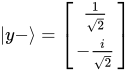
{\displaystyle |y-\rangle ={\begin{bmatrix}{\frac {1}{\sqrt {2}}}\\-{\frac {i}{\sqrt {2}}}\end{bmatrix}}}
密度矩陣:
ϱ
y
−
=
|
y
−
⟩
⟨
y
−
|
=
[
1
2
−
i
2
]
[
1
2
i
2
]
=
[
1
2
i
2
−
i
2
1
2
]
{\displaystyle \varrho _{y-}=|y-\rangle \langle y-|={\begin{bmatrix}{\frac {1}{\sqrt {2}}}\\-{\frac {i}{\sqrt {2}}}\end{bmatrix}}{\begin{bmatrix}{\frac {1}{\sqrt {2}}}&{\frac {i}{\sqrt {2}}}\end{bmatrix}}={\begin{bmatrix}{\frac {1}{2}}&{\frac {i}{2}}\\-{\frac {i}{2}}&{\frac {1}{2}}\end{bmatrix}}}
。
完全隨機粒子束的量子態不是純態,它可以由50%
|
z
+
⟩
{\displaystyle |z+\rangle }
|
z
−
⟩
{\displaystyle |z-\rangle }
ϱ
=
1
2
ϱ
z
+
+
1
2
ϱ
z
−
=
1
2
[
[
1
0
0
0
]
+
[
0
0
0
1
]
]
=
[
0.5
0
0
0.5
]
{\displaystyle \varrho ={\frac {1}{2}}\varrho _{z+}+{\frac {1}{2}}\varrho _{z-}={\frac {1}{2}}\left[{\begin{bmatrix}1&0\\0&0\end{bmatrix}}+{\begin{bmatrix}0&0\\0&1\end{bmatrix}}\right]={\begin{bmatrix}0.5&0\\0&0.5\end{bmatrix}}}
。 它也可以由50%
|
x
+
⟩
{\displaystyle |x+\rangle }
|
x
−
⟩
{\displaystyle |x-\rangle }
ϱ
=
1
2
ϱ
x
+
+
1
2
ϱ
x
−
=
1
2
[
[
0.5
0.5
0.5
0.5
]
+
[
0.5
−
0.5
−
0.5
0.5
]
]
=
[
0.5
0
0
0.5
]
{\displaystyle \varrho ={\frac {1}{2}}\varrho _{x+}+{\frac {1}{2}}\varrho _{x-}={\frac {1}{2}}\left[{\begin{bmatrix}0.5&0.5\\0.5&0.5\end{bmatrix}}+{\begin{bmatrix}0.5&-0.5\\-0.5&0.5\end{bmatrix}}\right]={\begin{bmatrix}0.5&0\\0&0.5\end{bmatrix}}}
。 另外,它還可以由50%
|
y
+
⟩
{\displaystyle |y+\rangle }
|
y
−
⟩
{\displaystyle |y-\rangle }
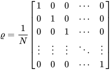
一般而言,完全隨機粒子束的
N
×
N
{\displaystyle N\times N}
ϱ
{\displaystyle \varrho }
[ 8] : 186
ϱ
=
1
N
[
1
0
0
⋯
0
0
1
0
⋯
0
0
0
1
⋯
0
⋮
⋮
⋮
⋱
⋮
0
0
0
⋯
1
]
{\displaystyle \varrho ={\frac {1}{N}}{\begin{bmatrix}1&0&0&\cdots &0\\0&1&0&\cdots &0\\0&0&1&\cdots &0\\\vdots &\vdots &\vdots &\ddots &\vdots \\0&0&0&\cdots &1\\\end{bmatrix}}}
。
对于一组能量本征态
|
ψ
n
⟩
{\displaystyle |\psi _{n}\rangle }
ρ
=
∑
n
ω
n
|
ψ
n
⟩
⟨
ψ
n
|
{\displaystyle \rho =\sum _{n}\omega _{n}|\psi _{n}\rangle \langle \psi _{n}|}
其中
p
n
=
exp
(
−
E
n
/
k
T
)
/
Z
{\displaystyle p_{n}=\exp(-E_{n}/kT)/Z}
Z
=
∑
n
exp
(
−
E
n
/
k
T
)
{\displaystyle Z=\displaystyle {\textstyle \sum _{n}}\exp(-E_{n}/kT)}
配分函数 。对于不含时哈密顿算符,热平衡的混态是不随时间演化的。[ 10]
薛丁格方程式描述純態怎樣隨著時間流逝而演化,馮諾伊曼方程式描述密度算符怎樣隨著時間流逝而演化。實際而言,這兩種方程式等價,因為它們彼此都可以推導出對方。假設,在時間
t
0
{\displaystyle t_{0}}
ρ
(
t
0
)
=
∑
i
w
i
|
ψ
i
(
t
0
)
⟩
⟨
ψ
i
(
t
0
)
|
{\displaystyle \rho (t_{0})=\sum _{i}w_{i}|\psi _{i}(t_{0})\rangle \langle \psi _{i}(t_{0})|}
其中,量子系統在時間
t
0
{\displaystyle t_{0}}
|
ψ
i
(
t
0
)
⟩
{\displaystyle |\psi _{i}(t_{0})\rangle }
w
i
{\displaystyle w_{i}}
假若不攪擾這量子系統,則機率
w
i
{\displaystyle w_{i}}
t
{\displaystyle t}
|
ψ
i
(
t
)
⟩
{\displaystyle |\psi _{i}(t)\rangle }
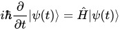
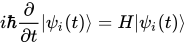
含時薛丁格方程式
i
ℏ
∂
∂
t
|
ψ
i
(
t
)
⟩
=
H
|
ψ
i
(
t
)
⟩
{\displaystyle i\hbar {\frac {\partial }{\partial t}}|\psi _{i}(t)\rangle =H|\psi _{i}(t)\rangle }
其中,
ℏ
{\displaystyle \hbar }
H
{\displaystyle H}
哈密頓算符 。
所以,馮諾伊曼方程式表示為[ 11] [ 12]
i
ℏ
∂
∂
t
ρ
(
t
)
=
∑
i
w
i
(
H
|
ψ
i
(
t
)
⟩
⟨
ψ
i
(
t
)
|
−
|
ψ
i
(
t
)
⟩
⟨
ψ
i
(
t
)
|
H
)
=
−
[
ρ
,
H
]
{\displaystyle {\begin{aligned}i\hbar {\frac {\partial }{\partial t}}\rho (t)&=\sum _{i}w_{i}(H|\psi _{i}(t)\rangle \langle \psi _{i}(t)|-|\psi _{i}(t)\rangle \langle \psi _{i}(t)|H)\\&=-[\rho ,H]\\\end{aligned}}}
; 其中,方括弧代表對易算符 。
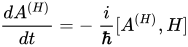
注意到只有當採用薛丁格繪景時(必須採用薛丁格繪景來計算密度算符)這方程式才成立,雖然這方程式看起來很像海森堡繪景的海森堡方程式,唯一差別是關鍵的正負號:
d
A
(
H
)
d
t
=
−
i
ℏ
[
A
(
H
)
,
H
]
{\displaystyle {\frac {dA^{(H)}}{dt}}=-\ {\frac {i}{\hbar }}[A^{(H)},H]}
其中,
A
(
H
)
{\displaystyle A^{(H)}}
在海森堡繪景裏,密度算符與時間無關,正負號差別確使期望值
⟨
A
⟩
{\displaystyle \langle A\rangle }
[ 註 4]
假若哈密頓算符不含時,則可從馮諾伊曼方程式推導出
ρ
(
t
)
=
e
−
i
H
t
/
ℏ
ρ
(
0
)
e
i
H
t
/
ℏ
{\displaystyle \rho (t)=e^{-iHt/\hbar }\rho (0)e^{iHt/\hbar }}
對於兩體純態系統,馮諾伊曼熵
σ
{\displaystyle \sigma }
a
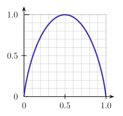
i
{\displaystyle a_{i}}
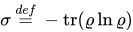
在量子統計力學(quantum statistical mechanics)裏,馮諾伊曼熵(von Neumann entropy)是經典統計力學關於熵 概念的延伸。對於密度矩陣為
ϱ
{\displaystyle \varrho }
[ 13] : 301
σ
=
d
e
f
−
t
r
(
ϱ
ln
ϱ
)
{\displaystyle \sigma \ {\stackrel {def}{=}}\ -\mathrm {tr} (\varrho \ln \varrho )}
這公式涉及到矩陣對數(logarithm of a matrix),似乎很難計算,[ 註 5]
ρ
{\displaystyle \rho }
[ 8] : 186–188
ρ
=
∑
i
a
i
|
a
i
⟩
⟨
a
i
|
{\displaystyle \rho =\sum _{i}a_{i}|a_{i}\rangle \langle a_{i}|}
其中,
|
a
i
⟩
{\displaystyle |a_{i}\rangle }
本徵值 為
a
i
{\displaystyle a_{i}}
本徵態 ,所有
|
a
i
⟩
{\displaystyle |a_{i}\rangle }
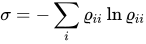
因此,可以將密度矩陣
ϱ
{\displaystyle \varrho }
ϱ
{\displaystyle \varrho }
σ
=
−
∑
i
ϱ
i
i
ln
ϱ
i
i
{\displaystyle \sigma =-\sum _{i}\varrho _{ii}\ln \varrho _{ii}}
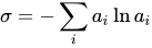
馮諾伊曼熵
σ
{\displaystyle \sigma }
σ
=
−
∑
i
a
i
ln
a
i
{\displaystyle \sigma =-\sum _{i}a_{i}\ln a_{i}}
從這形式,可以推論馮諾伊曼熵與經典信息論 裏的夏農熵 (Shannon entropy)相關。[ 13]
在這裏,可以視每一個本徵值
a
i
{\displaystyle a_{i}}
|
a
i
⟩
{\displaystyle |a_{i}\rangle }
lim
a
→
0
a
log
a
=
0
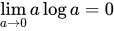
{\displaystyle \lim _{a\to 0}a\log a=0}
因此,可以採用約定
0
log
0
=
0
{\displaystyle 0\log 0=0}
純態的馮諾伊曼熵為零,因為其密度矩陣對角化之後,只有一個元素為1,其它均為0。即所有對角元素
a
i
{\displaystyle a_{i}}
a
i
=
0
{\displaystyle a_{i}=0}
ln
a
i
=
0
{\displaystyle \ln a_{i}=0}
完全隨機混合態的
N
×
N
{\displaystyle N\times N}
σ
{\displaystyle \sigma }
σ
=
−
∑
i
1
N
ln
1
N
=
ln
N
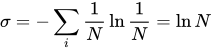
{\displaystyle \sigma =-\sum _{i}{\frac {1}{N}}\ln {\frac {1}{N}}=\ln N}
假若,將馮諾伊曼熵視為量子系統失序現象的一種量度,則純態擁有最小的馮諾伊曼熵
0
{\displaystyle 0}
ln
N
{\displaystyle \ln N}
每一次做投影測量,馮諾伊曼熵都會增加,永遠不會減少,但是,對於廣義測量(generalized measurement),馮諾伊曼熵可能會減少。[ 14] [ 15] 波函數塌縮 。實際而言,相當反直覺地,投影測量這動作抹除了複合系統的量子相干性 。更詳盡內容,請參閱條目量子退相干 。
一個量子系統的子系統可以從混合態改變為純態,但是所附出的代價是其它部分的馮諾伊曼熵會增加,就好似將一個物體放進冰箱來降低其熵 ,冰箱熱交換器外的空氣會變暖,而所增加的熵會比物體所減少的熵更多。更詳盡內容,請參閱條目熱力學第二定律 。
玻恩法則(Born rule)
格里森定理(Gleason's theorem)
密度泛函理論
^ 對於本徵態
|
a
i
⟩
{\displaystyle |a_{i}\rangle }
Λ
(
a
i
)
{\displaystyle \Lambda (a_{i})}
|
ψ
⟩
{\displaystyle |\psi \rangle }
|
a
i
⟩
{\displaystyle |a_{i}\rangle }
Λ
(
a
i
)
|
ψ
⟩
=
|
a
i
⟩
⟨
a
i
|
ψ
⟩
=
c
i
|
a
i
⟩
{\displaystyle \Lambda (a_{i})|\psi \rangle =|a_{i}\rangle \langle a_{i}|\psi \rangle =c_{i}|a_{i}\rangle }
c
i
{\displaystyle c_{i}}
|
a
i
⟩
{\displaystyle |a_{i}\rangle }
|
ψ
⟩
{\displaystyle |\psi \rangle }
^ 給定兩個規範正交基
{
|
a
i
⟩
}
,
{
|
b
i
⟩
}
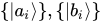
{\displaystyle \{|a_{i}\rangle \},\{|b_{i}\rangle \}}
W
{\displaystyle W}
tr
(
W
)
=
∑
i
⟨
a
i
|
W
|
a
i
⟩
=
∑
i
,
j
⟨
a
i
|
b
j
⟩
⟨
b
j
|
W
|
a
i
⟩
=
∑
i
,
j
⟨
b
j
|
W
|
a
i
⟩
⟨
a
i
|
b
j
⟩
=
∑
j
⟨
b
j
|
W
|
b
j
⟩
{\displaystyle \operatorname {tr} (W)=\sum _{i}\langle a_{i}|W|a_{i}\rangle =\sum _{i,j}\langle a_{i}|b_{j}\rangle \langle b_{j}|W|a_{i}\rangle =\sum _{i,j}\langle b_{j}|W|a_{i}\rangle \langle a_{i}|b_{j}\rangle =\sum _{j}\langle b_{j}|W|b_{j}\rangle }
^ 3.0 3.1 在量子退相干 裏,約化密度算符 代表的是反常混合物,它不能被視為處於某個未知的純態;它是依賴環境與系統之間的相互作用使得所有的非對角元素趨於零,實際而言,這些非對角元素所表現的量子相干性 已被遷移至環境,只有從整個密度算符才能查覺到這量子相干性的存在。[ 6] : 48–49
^ 在薛丁格繪景裏,純態隨著時間而演化的形式為
|
ψ
i
(
t
)
⟩
=
e
−
i
H
(
t
−
t
0
)
|
ψ
i
(
t
0
)
⟩
{\displaystyle |\psi _{i}(t)\rangle =e^{-iH(t-t_{0})}|\psi _{i}(t_{0})\rangle }
ρ
(
t
)
=
∑
i
w
i
|
ψ
i
(
t
)
⟩
⟨
ψ
i
(
t
)
|
=
∑
i
w
i
(
|
ψ
i
(
t
0
)
⟩
e
i
H
(
t
−
t
0
)
e
−
i
H
(
t
−
t
0
)
⟨
ψ
i
(
t
0
)
|
)
=
∑
i
w
i
(
|
ψ
i
(
t
0
)
⟩
⟨
ψ
i
(
t
0
)
|
)
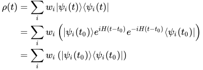
{\displaystyle {\begin{aligned}\rho (t)&=\sum _{i}w_{i}|\psi _{i}(t)\rangle \langle \psi _{i}(t)|\\&=\sum _{i}w_{i}\left(|\psi _{i}(t_{0})\rangle e^{iH(t-t_{0})}e^{-iH(t-t_{0})}\langle \psi _{i}(t_{0})|\right)\\&=\sum _{i}w_{i}\left(|\psi _{i}(t_{0})\rangle \langle \psi _{i}(t_{0})|\right)\\\end{aligned}}}
。
^ 矩陣對數(logarithm of a matrix)也是矩陣;後者的矩陣指數等於前者。這是純對數 的推廣。這運算是矩陣指數的反函數 。並不是所有矩陣都有對數,有些矩陣有很多個對數。
^ von Neumann, John, Wahrscheinlichkeitstheoretischer Aufbau der Quantenmechanik, Göttinger Nachrichten, 1927, 1 : 245–272 ^ 2.0 2.1 Ballentine, Leslie. Quantum Mechanics: A Modern Development 2nd, illustrated, reprint. World Scientific. 1998. ISBN 9789810241056. ^ Fano, Ugo, Description of States in Quantum Mechanics by Density Matrix and Operator Techniques, Reviews of Modern Physics, 1957, 29 : 74–93, Bibcode:1957RvMP...29...74F doi:10.1103/RevModPhys.29.74 ^ 4.0 4.1 4.2 4.3 Laloe, Franck, Do We Really Understand Quantum Mechanics, Cambridge University Press, 2012, ISBN 978-1-107-02501-1 ^ Griffiths, David J., Introduction to Quantum Mechanics (2nd ed.), Prentice Hall, 2004, ISBN 0-13-111892-7 ^ 6.0 6.1 6.2 Maximilian A. Schlosshauer. Decoherence: And the Quantum-To-Classical Transition. Springer Science & Business Media. 1 January 2007. ISBN 978-3-540-35773-5. ^ Bernard d' Espagnat. Conceptual Foundations of Quantum Mechanics. Advanced Book Program, Perseus Books. 1999. ISBN 978-0-7382-0104-7. ^ 8.0 8.1 8.2 8.3 Sakurai, J. J.; Napolitano, Jim, Modern Quantum Mechanics 2nd, Addison-Wesley, 2010, ISBN 978-0805382914 ^ Dirac, P. A. M. Note on Exchange Phenomena in the Thomas Atom. Mathematical Proceedings of the Cambridge Philosophical Society. 2008, 26 (3): 376. Bibcode:1930PCPS...26..376D doi:10.1017/S0305004100016108 ^ {S. VanEnk, "Mixed states and pure states," [Online Note]. University of Oregon. Available: https://pages.uoregon.edu/svanenk/solutions/Mixed_states.pdf (页面存档备份 ,存于互联网档案馆 ) [Accessed: September 25, 2023]}
^ Breuer, Heinz; Petruccione, Francesco, The theory of open quantum systems: 110, ISBN 9780198520634 ^ Schwabl, Franz, Statistical mechanics: 16, 2002, ISBN 9783540431633 ^ 13.0 13.1 Bengtsson, Ingemar; Zyczkowski, Karol. Geometry of Quantum States: An Introduction to Quantum Entanglement 1st. ^ Nielsen, Michael; Chuang, Isaac, Quantum Computation and Quantum Information, Cambridge University Press , 2000, ISBN 978-0-521-63503-5 ^ Everett, Hugh, The Theory of the Universal Wavefunction (1956) Appendix I. "Monotone decrease of information for stochastic processes" , The Many-Worlds Interpretation of Quantum Mechanics, Princeton Series in Physics, Princeton University Press: 128–129, 1973, ISBN 978-0-691-08131-1
系综
微正则系综
正则系综
巨正则系综
等温等压系综
Isoenthalpic–isobaric Open 統計熱力學 配分函数 状态方程 熵
Sackur–Tetrode equation Tsallis entropy Von Neumann entropy 近独立粒子 统计场论
共形場論
Osterwalder–Schrader axioms 量子统计力学
正则系综
密度矩陣 Gibbs measure 配分函数 Weyl quantization 斯莱特行列式 參見
背景 基礎 表述 方程 空間幾何 詮釋
量子力學詮釋 量子貝葉斯詮釋 一致性历史
哥本哈根詮釋 德布罗意-玻姆理论
系綜詮釋
隱變量理論
多世界诠释 客觀坍縮理論
量子邏輯 關係性量子力學
隨機量子力學 交易詮釋
宇宙学诠释 實驗
阿弗沙爾實驗
貝爾測試實驗 冷原子實驗室 戴維森-革末實驗
延遲選擇量子擦除實驗
雙縫實驗 法蘭克-赫茲實驗 萊格特 - 加爾格不等式 馬赫-曾德爾干涉儀
伊利澤-威德曼炸彈測試問題
波普尔实验
量子擦除實驗
薛定谔猫 施特恩-格拉赫实验 惠勒延迟选择实验 量子纳米科学
量子貝葉斯詮釋 量子生物学 量子微積分 量子化学 量子混沌 量子認知 量子宇宙學
量子微分 量子動力學 量子演化 量子幾何 量子群
測量問題 量子概率 量子隨機演算 量子時空 量子技術
量子演算法
量子放大器 量子總線 量子点
量子通道 量子線路
量子复杂性理论
量子计算机
量子密碼學 量子電子學 量子誤差校正 量子成像
量子圖像處理 量子信息
量子密鑰分發
量子邏輯 量子閘 量子機 量子機器學習
量子超材料 量子計量學 量子网络 量子神經網絡 量子光学 量子編程
量子傳感器 量子模拟器
量子隱形傳態 進階研究 物理學者